View - IRCCyN - Ecole Centrale de Nantes

qetIt
IEEE TRANSACTIONS ON CONTROL SYSTEMS TECHNOLOGY, VOL. 2, NO. 4, DECEMBER 1994 371
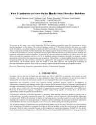
Experimental Results for the End-Effector
Control of a Single Flexible Robotic Arm
Y. Aoustin, C. Chevallereau, A. Glumineau, and C. H. Moog, Member, IEEE
Abstract-Various control schemes for a single flexible robot perturbations, sliding mode techniques, as well as hybrid issues
arm are considered in this paper. They require a limited amount will be considered in Section 111. The purpose is not to survey
of on-line computations. All trials are performed on the physical
the literature on the subject but to display the features of
process and embody a conclusive, although partial, comparison
for this kind of single axis robot. They are representative of each considered control law and to give the experimental
some major applied research directions which captured the at- results obtained on a single plant. Control methods as adaptive
tention of many researchers throughout the 1980’s. Some general methods and generalized predictive control [14], [17], [26] are
conclusions are derived.
not considered herein. Some of the control methods considered
in the paper can be found in the current literature but the
I. INTRODUCTION
experimentation is seldom performed on the same process.
As far as system analysis is concerned, the end-point of
T
HE control of mechanical systems and particularly of
robotic manipulators is an active applied research area.
After the era of rigid robotics, major research activity was
devoted to improve dynamic performances and to reduce
the mass of robotic systems. Design solutions to minimize
the effects of the elastic displacements of large amplitude
and light robots have been used by choosing, for instance,
materials which are able to stiffen the structure or to damp the
vibrations [20]. Another solution consists in developing openloop
strategies, using nonexciting trajectories which minimize
the elastic displacements of the structure [29],[31]. Since it
is not possible to take disturbances into account with such
methods, the so-called active closed-loop control of structural
flexibilities, including elastic joints, received an increasing
interest.
Different approaches are available for designing the control
laws. The controller may be obtained from the distributed parameter
model of the flexible robot arms [35], from a discrete
model in space and in time [27], or from a discrete model
in space and continuous in time as done in the mainstream
of the current literature. This last method is based on the
modal decomposition [30] or on the finite element scheme [9],
[34]. The model used in the sequel was obtained from a finite
element decomposition. A main constraint for the model is that
it has to be used real time in the control-loop. A few years
ago, researchers began studying single-link flexible robots,
[37], as well as robots possessing elastic joints [3], [16], [33].
Certain control schemes are now studied for multilink robots
and are getting increasing interest [l], [2],[13], [15], [21],
[24],[38]. The goal of this paper is to analyze experimental
results on a single arm of some of these control policies.
Classical PID controllers, nonlinear control structures, singular
Manuscript received July 15, 1993; revised December 14, 1993. Recommended
by Associate Editor, D.W. Clarke. This work was supported in part
by CNRS through the “Groupement de Recherche Autornatique.”
The authors are with the Laboratoire d’Automatique de Nantes, Unitee
Associke au CNRS 823, Ecole Centrale de Nantes. Universiti de Nantes, 1
Rue de la Noe, 44072 Nantes Cedex 03. France.
IEEE Log Number 9403413.
a flexible beam is representative of a nonlinear system with
unstable zero dynamics [7], [23], a so-called nonminimal phase
system. For such reasons, recent results in systems theory [22]
may be involved when considering the control problem of the
end-point of a flexible beam.
10634536/94$04 .Do Q 1994 IEEE
11. MATHEMATICAL MODEL, SYSTEMS DESCRIFTION
The modeling of flexible structures has been studied by
many researchers. The infinite dimension of the problem is
generally solved by using a discretization method. It may be
the finite element model or the modal approach. In this paper,
a finite element model is used where the elastic displacements
of the structure are referred to the rigid configuration of each
link. For a robot with n, joints, the dynamic model is written
as follows
where
- A is the mass matrix, while B(q: q ) are Coriolis and
centrifugal forces.
- q = [qPt ~ is the vector of the rigid and elastic
degrees of freedom, we note that dim(q,) = n,. and
dim(qe) = ne.
- q and q are respectively the velocity and acceleration
vectors.
- K contains the stiffness terms.
- G(q) contains the gravity terms. As we study a planar
flexible robot where gravity is compensated, G(q) = 0.
- L,r, is the vector of the generalized torques or forces
(dimension n = n, + ne).
- Ta is the vector of the actuators torques (dimension: nT).
One finite element per link is used. It has been proved in [8]
that a single finite element is sufficient to correctly describe the
dynamic behavior of the robot. Moreover, the two first modes,
either with clamped limit condition or simply supported limit
conditions, are well described. This is due to the important

312 IEEE TRANSACTIONS ON CONTROL SYSTEMS TECHNOLOGY, VOL. 2, NO. 4, DECEMBER 1994
TABLE I
NUMERICAL DATA OF T€E ROBOTIC SYSTEM
A7
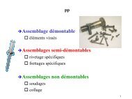
Fig. 1. blexible robot.
concentrated mass at the end-point of the link. In the case of a
plane flexible robot, one gets three variables for each link: Oi is
the rigid degree of freedom, VB~
and 8gi are the displacement
and the rotation of the terminal section. They represent the
degrees of freedom of the robot (see Fig. 1, with one flexible
link).
Vector q represents the rigid and elastic variables, q =
[e VB OB]'. This model is general. It can describe any type
of robot structure. The dynamic model is almost the same as
for a rigid robot. The main difference is that for a rigid robot
La is an (n, x n,) identity matrix. The expression of matrices
A, B, K are defined in [lo], and they are given for a one-link
robot as shown by A at the bottom of the page and
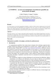
Fig. 2. The experimental robat.
and 2.43 Hz. They correspond to zeros of the transfer of the
approximate linearized model as presented in Section 111-C
between the torque and the rigid variable. The experimental
(planar) robot is shown in Fig. 2. The rotational joint is parallel
to the direction of gravity. The extremity of the link has air
bearings to avoid gravity effects.
The mechanical characteristics of the robot under interest
were identified on the plant in Table I.
In the experimental device, the first vibration mechanical
structural modes of our robot are at frequencies 0.264 Hz
111. EXPERIMENTED CONTROL SCHEMES
The physical process has some differences with the mathematical
model given in Section IT, higher frequency mechanical
modes as well as constant friction are unmodeled.
Coulomb friction is, however, identified, and its average value
equals 0.140 Nm on the actuator output axis. Unfortunately,
this friction factor depends of the axis position. So, its compensation
is a difficult matter. A continuous model is used
to define the control law using a HP 1000 A 900 computer
and the sampling period is 5 ms. The hardware architecture
is presented in Fig. 3.
The sensors are a tachometer to measure 8, an encoder
to measure 6, and strain gauges which 'are located on the
links to measure deformation of the link in two particular
places. So the elastic variables and their time derivatives
are computed, from the strain-gauges information, by using
-
p LI+-
"31
A= p I + -SL + m,L
SL3
+~,(L*+V~)+J~+J~ p +mcL - p y + J ~
[ z'o 2]
SL3
- P m + JB
-p [-+-
:o-
SL3
4,+15]+JB
ll;foLz]
2LI

AOUSTIN et al.: RESULTS FOR THE
the finite element model. This computation is valid only if
V, is within a range of 10% of the length of the arm.
This yields the choice of the reference trajectory adopted
in the rest of this paper. Analogical antialiasing filters and
numerical filters limit spillover noise on the measurements.
The input torque delivered by the electric actuator is bounded
to 2 Nm. The results given in the rest of this section are
obtained from the implementation on the robot system. The
measurements are filtered after the first mode (at 0.3 Hz),
before the computation of the velocities d s and $b, to avoid
undesired high frequencies.
A. The Desired Trajectory
The desired trajectory for the end-effector of the link is a
fifth-order equation which is defined by
Yd(t) = yi + dr(t) (3.1)
where yi is the initial position, d is the displacement, yd is
the current desired position, and r(t) is a function of the time.
The desired positions of the elastic variables are zero since
the fulfillment of the trajectory yd(t) without stabilization of
the elastic variables is not acceptable; the orientation of the
end-effector would remain unstable.
To define a trajectory which is smooth and continuous in
position, velocity, and acceleration, we choose
END-EFFECTOR
CONTROL OF ROBOTIC ARM 373
Calculator
HPlwO AWO
-
1 ’ 7
C.A.D. : malogicdigital convertex
C.D.A. : digira-andogic converter
I.D. : counting card
Fig. 3. Hardware architecture.
Actuator 1
ARTIJS
“2wO
Tachymemc
dynamo
Encoder
Strain gauges
amplificator
gauges Link Strain
where T, is the expected duration of the motion. With this
equation, the desired velocity and acceleration at the initial
and final position are zero. T, is computed as a function of
the maximal admissible velocity and acceleration of the link.
This type of trajectory allows the definition of a desired
velocity and a desired acceleration during the whole time of
the displacement. They may eventually be used in the control
law. On the other hand, the elastic deflections are less excited
than by a step reference, and they have a more acceptable
response. This trajectory avoids saturation of the actuators at
initial conditions. These advantages justify its frequent use in
robotics. The tested trajectory is ‘yi = 0 rd, d = 1.57 rd, T, =
7.36 s.
B. PD Controller
Considering the position of the end-point (LO + VB), one
deals with a nonminimum phase system [7], [23] and the
PD control derived from this output (LO + V,) yields an
unstable closed-loop system. The rigid angle O as an output
defines a minimum phase system. A classical proportional and
derivative controller for this output has been tested and will be
used as reference in the controller performance comparison.
The best tuning of such a controller yields a response time
of about 13 s for a fifth-degree polynomial input; decreasing
this response time with another tuning causes serious troubles,
since the flexible modes would be activated and the dynamical
behavior of the end-effector of the robot would no longer be
acceptable. This tuning is Kp = 2 and K, = 7 in
-0.5 I I I
1’0 15 i0
tim*
Fig. 4. PD controller: Reference (- - - -, rn) and end-effector (-, rn) versus
time (3).
where Od is computed from Yd with 1’8 = 0. The break
frequency of this corrector is at low frequencies, so it acts like
a forward phase shift of 90 degrees for almost all frequencies.
In the next figures, the dotted line represents the desired
trajectory yd, the position of the end-effector, and the solid line
represents the measured variables. In Fig. 4, the end-effector
response (LO + VB) to the PD controller (3.2) is displayed and
the corresponding input torque is given in Fig. 5.
A slight modification of this control low is considered below
and is called “speed feedback” hereafter
In both cases, there is a static error which is due to the
friction effects. Usually it is possible to cancel this error using
an integral term. A compromise between the behavior of the
controller at low and high frequencies, however, has to be
sought. Some large overshoots, depending on the trajectories,
may appear with nonlinear systems. The flexibilities of the
robot considered in this paper are greater than standard flexibil-
Fa = Kp(ed - 0) + K,(dd - 6) (3.2) ities which occur in industrial applications. This implies some

374 IEEE TRANSACTIONS ON CONTROL SYSTEMS TECHNOLOGY, VOL. 2, NO, 4. DECEMBER 1994
2- C. LQR Controller
The torque is defined by
1-
ra = -Kv(q - qd) - Kp(q - qd) (3.4)
where K,, K, are (1 x 3) matrices; the measurement or
8 0-
8 estimation of all the state variables is necessary.
The gain matrices K, and K, are obtained from a LQR
method, minimizing the following criterion
-1-
-2 c=~~{(q-qd)'Ql(q-qd)+(q-Pd)*Q~(q-qd)
, , , .
Fig. 5. PD controller: Torque (-, .Vm) versus time (8).
J
r--------___-----______
1.5 -
lb lls ia
tima +r:Rr,)}dt (3.5)
,
where Q1, Qz, are semidefinite positive and R is definite positive.
Such a method ensures proper gain and phase margins.
The weighting matrices are associated to the state and control
variables and yield the computation of a state feedback. Thus
it is necessary to define a desired state trajectory, even if the
output is yd. To apply this method, we use an approximate
linearized model of the robot. We linearize the dynamics
around an equilibrium point of the robot so that q, = 0, and
q = 0. The linearized model that one obtains is independent
on the rigid variable B
-0.5 I I .
,
lb
lime
t
15 20
Fig. 6. Speed feedback: Reference (- - - -, m) and end-effector (-, m)
versus time (s).
The closed-loop behavior of the flexible robot is defined by
2- From the form of K and qd, K q can be replaced by
K(q - qd). The robot can be considered as three coupled
second-order systems submitted to the disturbance given by
1- the right-hand side of (3.7). The weighting matrices have
f 0-
been designed using the Bryson rule [6] so that the maximal
admissible torque and the maximal admissible deflection of
the link are respected
-1-
Q1 = diag(lO.l, 1): Q z = diag(l.1,l). R = 1
the corresponding solution is
-2- . , , ,
10 15 ' ' io K,= [3.16 - 5.83 4.531 and Kv=[6.27 5.16 - 0.741.
lime
Fig. 7. Speed feedback Torque (-, N. m) versus time (s).
So the control laws are
overshoots in several cases and in particular for PD control,
the situation would become worse with the adjunction of an
integral term. No integral action has been implemented. The
overshoot obtained with the PD controller (3.2) can eventually
be cancelled by modifying the tuning, but it was kept to
compare the controls (3.2) and (3.3). It is worthwhile to point
out a particular poor behavior which characterizes the above
PD controller, w.r.t. the next controllers, since it is heavily
sensitive to disturbance forces; when the robot is hit, some
severe oscillations will occur and be maintained. An extension
of such a PD controller design to a two-flexible link robot can
be done uniquely by considering independent arms.
or
ra = 3.16(ed - e) + 6.27(ed - e) + 5 .83~~
- 5.16V~ - 4.538B + 0.748~ (3.8)
ra = 3.16(~~ - e) - 6.278 + 5 .83~~ - 5.16VB
- 4.530~ + 0.748~. (3.9)
For the single link robot and in the experimental test, the
response of the control law (3.8) and the response of the
control law (3.9) are, respectively, displayed in Figs. 7 and
9. The advantage of this controller, w.r.t. the PD controller,
is that it remains insensitive to external disturbances. For an

AOUSTIN er ai.: RESULTS FOR THE END-EFFECTOR CONTROL OF ROBOTIC ARM 375
1.5
“i 1.5 /
1 I /
0.5
0.0
-0.5 , , , ,
10
time
15 d0
Fig. 8. LQR controller (Tal): Reference (- - - -. m) and end-effector (-,
rn) versus time (5).
-0.1 , I I , I
10 15 20
lime
Fig. 10.
versus time (s).
LQR controller (ra2): Reference(--, m) and end-effector (-, m)
-2 , , , ,
Fig. 9. LQR controller (Tal): Torque (-,
lb lh 2b
tima
.Vm) versus time (s).
-1
-2’ , , , z
Fig. 11.
10 15 20
time
LQR controller (ra2): Torque (-, .h‘m) versus time (5).
extension to a two-flexible link robot, the linearized model
depends on the configuration of the robot.
From (3.7) a LQR control yields a linear closed-loop system
subject to a “nonlinear disturbance.” A nonlinear control can
be introduced besides the LQR control for minimizing the
effect of the disturbance, so that the closed-loop behavior
approaches
or
6 -t Kvlq + Kpl(q - qd) = 0 (3.10)
(6- qd) + KvI(~
- ‘id) + Kpl(q - qd) = 0. (3.11)
Since there are nonlinear equations relating 8, VB, OB, and q,
neither (3.10) nor (3.11) can be exactly matched. So one looks
for the torques Ta which minimize the “distance” between the
real behavior of the robot and the desired behavior. The real
behavior of the robot is defined by (2.1)
4 = A(q)-’[Lara - B(q, 4) - Kq]. (3.12)
This “distance” is defined by the norm of the difference
between the values of q calculated by (3.10) and (3.12) or
(3.11) and (3.12). For instance, using (3.12) in the left-hand
side of (3.10), the criterion to minimize is
c1 = II{A-l[Lara - B(q, 4 - Kql + K”l4
+ Kpl(q- qd)>11*. (3.13)
This norm is
minimal for
ra = {A-’La}+{A-’(B(q, qj + Kqj
- Kv1c1- Kpl(q - qd)}. (3.14)
Since A-lL, is not invertible, full disturbance rejection is
not possible. With the nonlinear control law (3.14), the effect
of the disturbance on q is minimized, and from a mathematical
point of view, the disturbance is orthogonally projected onto
the kernel of (A(q)-IL,)+. Thus, in general, the effect of
the disturbance will be less important for the nonlinear control
law than for the case where the LQR linear control law only
is applied.
In [12], it is shown that the above LQR controller is improved
for multijoints robots, when a disturbance minimization
scheme is implemented. This control law reduces the variation
of A(q)-lL,K,, A(qj-’{L,K,+K} along the trajectories.
For completeness, this modification has been tested on the
single arm robot in the following way. It has not shown to
yield a significative benefit for our single link robot. As stated
at the beginning of this section, from the flexibility of the
robot, the speed of motion is not large and the nonlinear terms
are not dominant.
D. Feedback Linearization Techniques
From recent developments of nonlinear system theory, a
concept of zero dynamics has been defined [7], [23] and

376 IEEE TRANSACTIONS ON CONTROL SYSTEMS TECHNOLOGY, VOL. 2. NO. 4, DECEMBER 1994
shown to play a role that is quite similar to the linear case;
as a by-product, the standard exact linearization techniques
via feedback, correspond to the linear pole-zero cancellation
phenomenon. More precisely and in the particular case of
the robot, it is possible to perform the input-output feedback
linearization when considering the end-point position LO + V,
as output, but this control policy yields unstable unobservable
dynamics. The relative degree of this output function is two,
thus the unobservable subsystem has dimension four after
feedback linearization and is unstable for this particular choice
of output. Thus, elementary feedback linearization techniques
can be applied only on other outputs as the so-called rigid
variables, e.g., [ll].
The output 6’ has relative degree 2, then the rigid acceleration
is given by
= Lq = LA-l{L,r, - B(q,q) - Kq} (3.15)
with L = [l 0 01 and solve in Fa this equation to get
.. ..
0 = 0d - Ky(b - ed) - Kp(O - 6’d). (3.16)
I
1
30 5.00 15.0 20.0
T1O.O
Fig. 12. Feedback linearization of 8: 0 rigid angle (-, m) versus time (s).
This yields
ra = (LA-~L,)-~{&- K,(B - id) - ~ ~ - ( ed) 0
- LA-lB(q, q) - LA-lKq)}. (3.17)
For this control law, the matrix A, its inverse and the vector B
must be computed at each sampling time. The response of the
system is not sensitive to the second-order elastic terms of A
and B. This simplification reduces dramatically the complexity
of the computation of Fa which becomes
ra = o .o~q& + ~ ~ - e) ( + K,(& 0 - ~ e)}
+ 7.225 VBP - 0.0515 6’88’.
(0 - 0d) behaves as a second-order system and since its
initial condition is zero, Kp, and K, have no influence on
the simulation response; the rigid angle B perfectly tracks the
command.
Fig. 12 shows the behavior of 0 which is perfect whereas
nonasymptotically stable oscillations appear in the behavior of
the elastic variables. The displacement of the end-point of the
beam is not acceptable but is a nice practical illustration of
the notion of unstable transmission zero.
A conclusive remark for further application of exact feedback
linearization should go through a modeling of structural
damping (even if small) of the flexible variables which will
improve the behavior of the end-point (LO + V,) without
decreasing the performance on 6’. The major advantage of
this feedback linearization is the easy practical choice for
the tuning parameters Kp and K, characterizing the linear
second-order system. This is not the case for the design of
weighting matrices in a LQR method or for designing a PID
controller. Feedback linearization requires a good knowledge
of the model, however, and this is a task which is difficult to
fulfill, due in particular to the damping phenomena.
s
-’
u
In
m
a51
0
n,l
’ 0.00 5.00 15.0 20.0
TlO.O
Fig. 13. Feedback linearization of 8: end-effector (-, m) versus time (3).
E. Singular Perturbation Method
In robotics, singular perturbation theory is applied for
controlling the flexible joint robots [33] or the flexible link
robots [25], [30]. An overview of the subject is provided in
[19]. The so-called rigid variables are slow, and the elastic
variables result from the superposition of a slow mode and a
fast mode.
To apply the singular perturbation method to these problems,
the elastic forces are introduced as new state variables. In [331,
these new state variables are based on the product of a spring
term that represents the joint flexibilities, and the difference
occumng in the position of each link w.r.t. its actuator. The
actuator position is divided by the gear ratio. In [30], which
illustrates our problem, the author defines the elastic forces,
z = kq,: where 5 is a positive common scale factor such as
K = kK.

AOUSTIN et a[.: RESULTS FOR THE OF ROBOTIC END-EFFECTOR ARM CONTROL
311
The variables x2 and u can be decomposed in a slow and
fast part [36]. The torque which is applied to the robot to
track the trajectory induces a slow dynamics for the variable
x1 whereas x2 results from the superposition of a slow mode
xzS and a fast mode xzf
xz(t0) = XZf(0) + xzs(t0)
u(h) = Uf(0) fus(t0).
0 1
m' I
IO.00 5.00
T1O.O
Fig. 14. Feedback linearization of 8: Torque (-,
15.0 20.0
Tm) versus time (s).
I
The fast subsystem is given by
dxl
= EF(x1.x2f(T) +xzs:uf(~) + us,&) (3.22a)
(.-
=
G(XI! Xzf(T) + xzs, uf(T) + us: E ) (3.22b)
dr
where xis. and us are assumed to be constant.
Now it is possible to propose a computation of the two
control parts. We may begin by the slow control part us. To
compute us we can rewrite (3.21a) under the form (3.23)
One can write
B1 and BS have respectively the dimension (n, x I) and
(ne x 1).
Since the mass matrix is symmetric positive definite, its
inverse is also symmetric positive definite. Let them be defined
as
Remarks:
- When E equals to 0, A and W are uniquely function of
xls. The subscript "s" stands for the evaluation of the
different matrices at q, = 0.
- For one flexible link robot we can note that B1,
(qr, 0, qr, 0) and B~s(qr, O,qr> 0) are equal to 0.
is determined by the computed torque method for a
rigid robot requiring that the system tracks a desired
trajectory.
(3.18)
E is equal to &.
By writing the system (3.18) under the state form we obtain
(3.19a)
(3.19b)
x1 and xz are, respectively, joined to slow and fast variables
and are equal to
We choose the gain such as K,, = 2 6 to obtain a damping
factor that is equal to one. The knowledge of us allows to
determine xzS
Concerning the fast part uf. after some computations, (3.22b)
becomes
(3.20)
which correspond, respectively, to rigid and elastic variables;
u, the control term is, of course, Tu. We consider a slow
subsystem with the scale time (t) and a fast subsystem with
the scale time (T) [28], so that T = (t - to)/€. The slow
subsystem is obtained by setting E = 0. The n2 differential
equations (3.19b) become algebraic. We have now [4], [5]
(3.21a)
(3.21b)

378 IEEE TRANSACTIONS ON CONTROL SYSTEMS TECHNOLOGY, VOL. 2, NO, 4, DECEMBER 1994
Fig. 15. Singular perturbations controller: Reference (- - - -, m) and
end-effector (-, m) versus time (5).
Fig. 16. Singular perturbations controller: Torque (-, .Vm) versus time (3).
Then one deduces
= (1- KR1K-1A21sA;~s)~s - KR [:gel
Finally the numerical parameters of the computed torque
for one flexible link robot are
ra = 7.264[(& - o m(8 - id) - o.qe - ed)] + 0.4125 vB
+ 0.1547 VB - 0.2544 95 + 0.2078 8,. (3.27)
Note that in (3.27), in opposition to the other control laws,
there is no term depending on q,+, since the decomposition
into two subsystems neglects the couplings between slow and
fast variables. To verify the two-time scale separation of the
slow and fast closed-loop systems, one neglects the couplings
and the system (3.19) becomes linear. The dynamics of (3.28a)
must be much slower than those in (3.28b)
(3.28a)
(3.28b)
One chooses eigenvalues such that [18] X(AI~),,,~~ 5
X (E-~AZZ) min.
Fig. 14 displays a good trajectory tracking for the end-point
of the robot. The final position is reached in about 10 seconds,
however, there is a 2.5% static error. It is possible to add an
integral term in the control law, but it would increase the
overshoot on the end-point response. The computed torque
is comparable to the ones obtained with the other control
schemes. It satisfies the bounds on the maximal torque which
is equal to 2 Nm. The experiments show that the torque uf is
small with respect to us, this is usual in practice.
The singular perturbation method induces some model simplifications,
which yield in our case the design of simplified
Fig. 17. Shape
of the Sign1 function.
controllers. A simple-computed torque control is implemented
for the slow subsystem and a restricted state feedback is used
for the fast subsystem. The main advantage of this method
(w.r.t. Section 111-D) is to decrease the on-line computations,
and this point becomes particularly crucial for multijoint
robots.
F. Sliding Modes Techniques
Sliding modes controllers are quite appealing since they
are designed for robust control which is of major importance
in practical experiments. Recall the basic and fundamental
principles. Choose a so-called sliding surface .(x), which
can be considered as an output whose relative degree equals
one, Le., di(a! u)/du # 0. Consider the Lyapunov function
V(x) = 1/2s2(2) and solve in 'LL
V(x,u) 5 0. (3.29)
The goal is to design a control u which drives the state 2
of the system onto the surface s(z) = 0. The equilibrium on
the sliding surface has to yield the physical control objectives.
Besides this constraint, the practical implementation of such
a control is feasible only if 9(2) defines a minimum phase
system when considered as an output, otherwise the motion
restricted on the surface s(x) = 0 is unstable.
To solve (3.29), it is possible to write u = .ueq + un
where ueq is the solution V(z,u) = 0. Set V(x! u) =
VI(.) + v2(x)u, then
ueq = -V1(.)/Vz(.)
and a class of solutions to (3.29) u, is given by
un = -k sign(Vz(z)), k > 0.
....

:I /r\
1 . , . , . , . . . . . , . . . .
dbw
Fig. 19. Sliding modes techniques: Torque (-, A‘mj versus rime (8).
There is bang-bang type term un in the control which does
not cause a major trouble in the numerical simulation when
applied to the model of the robot given in Section 11. For the
practical implementation on the physical system, however, the
actuators can not perform instantaneous commutations. Due
to the chattering phenomenon, the results are not as expected.
This can be largely improved by doing the computation of
sliding mode controller which takes into account a model of
the actuators, even very elementary. This is done next since it
is particularly crucial in this section. The actuator is modeled
by a first order system.
Let s(z) = - 0,) + PVB + 8. (3.30)
The signs of parameters ctl and ,f3 determine the stability
of the closed-lopp system and their values the response time.
In the frame of sliding modes, the so-called equivalent control
ueq solves the equation i = 0 and thus, is the feedback control
which linearizes the “output” s(x)
ueq =
(a(id - 8) - /?I&)(V; + 1.65E - 3)
0.147
(7.3~5 - 38B - 1.06V~)e’ - 2.3188 f
-
6.16V~
0.147
(3.31)
with cz = 0.35,,8 = -2.
As recalled previously, the standard sliding modes technique
induces some undesirable chattering in the control. These high
frequency commutations are created when the state trajectory
of the System is close to the sliding surface and then the
value of sign function changes often. To decrease the effect
of chattering, some classical issues are experimented in the
modification of the u, term of the control. The first one is
as follows
u, = -k sign(Vz(z)) = -k sign(s(a)): k 2 0,
if s(z) e] - E. +E[, E = constant
un = 0: if s(z) E] - E, +E[.
The parameter E is determining for the chattering in the closedloop
system. A too-large value of E, however, will decrease
the performance. To decrease the chattering even more, we
will adopt an alternative method for designing the u, term
of the control. As done in [32], we use another continuous
function, say Signl, to replace the sign function. The results
are obtained with a = 0.35, /3 = -2, and E = 0.035.
Concerning the tuning of the controller, the sliding modes
scheme has the same level of simplicity as the exact feedback
linearization techniques (Section 111-D) but is more robust.
The main point which is argued in this context concerns
the definition of the sliding surface equation s(.c). This is
solved in the robot system by defining a “minimum phase”
output function. Despite the u,, term of the control has been
smoothened, the control is still sensitive to the noise on the
variable Vg which was filtered.
IV. CONCLUSION
The strength of the paper relies in the experimental results
comparison performed (in a partial way) for various nonadaptive
control schemes. Five controllers have been tested on a
robot whose flexibilities are greater than standard flexibilities
which occur in industrial applications. The goal of this study
is to derive some general conclusions valid for a whole class
of systems as flexible robots. The plant is not an industrial
robot in the sense that its flexibility is intentionally large.
The reference trajectory has been chosen to avoid physical
limitations of the drive; otherwise, on the one hand, the
comparison of the different methods would be meaningless
and, on the other hand, one could not avoid permanent
deformations of the link.
For feedback linearization and LQR with disturbance minimization,
an on-line matrix inversion is necessary if the matrix
A described in Section I1 is used. A constant matrix A requires
only an off-line inversion to compute the torque r. For a
multilinks robot, a constant matrix A can not be used. Note
that an on-line matrix inversion for All is also necessary in
the case of several joints with the singular perturbation method
to compute Xas.
In the present state of the investigations, the singular perturbations
method appears to provide the best tracking of the
reference trajectory. This is a byproduct of the time scale
decomposition which yields a direct tuning of the 8 dynamics
which is not disturbed by the flexible modes. There is a
steady-state error, however, which can be eventually improved
by switching to another control scheme designed for the
regulator problem. The sliding modes technique can eventually

380 IEEE TRAKSACTIONS ON CONTROL SYSTEMS TECHNOLOGY, VOL. 2, NO. 4, DECEMBER 1994
TABLE I1
be improved for the tracking purpose by including a constraint
on 6’ in the sliding surface definition. The parameters of any
control scheme have to be tuned in a final phase on the
physical process, and this point becomes a real difficulty for
the practical implementation of the LQR method since many
parameters are involved in the weighting matrices of the cost
function.
Future work should consider an uncertainty on a load added
at the end-effector of the beam. This was partly done for
the sliding mode control and that it showed to be able to
cope with such an heavy uncertainty. No significant change of
the dynamical behavior is noticed for a load mass up to 500
g. Some persistent oscillations appear when the mass of the
load is as large as 1 kg. More generally, the different control
methods studied herein feature robustness since they show
their ability to cope with identification errors and uncertainties
which have not been modeled as Coulomb friction which is
not constant along the trajectory. The conclusions from our
experiments are summarized in Table 11.
The purpose was to test some controllers which are fully
designed off line in the sense that there is no heavy computational
task to be performed on line. The latter discussion
could be started when considering, for instance, some larger
adaptive control structures which could recompute the tuning
parameters of the various controllers to improve their robustness
properties. In such a situation, some new severe problems
would arise, however, such as the stability of the overall
structure. So, it is important to notice the intrinsic advantages
and limits of each elementary controller as done in Section 111.
The extension to rnultilink robots is feasible in principle
for all control procedures. Except for PD control, it is natural
to perform analysis on the global system. For a PD, tuning
consists in designing controller parameters link by link.
REFERENCES
Y. Aoustin, P. Chedmail, C. Chevallereau, A. Froment, and M. Faillot,
“Control of a robot with flexible links,” in Pmc. Int. Conf ICAR ‘91,
Pise, Italy, 1991, pp. 114-1 17.
Y. Aoustin and C. Chevallerean, “The singular perturbation control
of a two-flexible-link robot,” in Proc. IEEE ICRA, Atlanta, 1993, pp.
737-742.
A. Benallegue, “Contribution d la cornrnande dynamique adaptative des
robots rnanipulateurs rapides,” Ph.D. dissertation, Paris VI Univ., 1991.
P. Borne, G. Dauphin-Tanguy, 3. P. Richard, F. Rotella, and I. Zambettakis,
“Collection mkthod et techniques de I’ingenieur,” in Commande
et Oprimisation des Processus, Editions Technip, Paris, 1990.
P. Borne, G. Dauphin-Tanguy, J. P. Richard, F. Rotella, and I. Zambettakis,
“Collection mdthodes et techniques de l’ingdnieur,” Moddisarion
et IdenfiJication des Processus, Editions Technip, Paris. 1992.
A. E. Bryson, Jr. and Y. C. Ho, Applied Optimal Control. Hemisphere
Publishing, 1992, pp. 328-338.
C. I. Byrnes and A. Isidori, “Local stabilization of minimum-phase
nonlinear systems,” Syst. Contr. L eft, vol. 11, pp. 9-17, 1992.
P. Chedmail, “Synthkse de robots et de sites robotisks-moddlisation de
robots souples,” Ph.D. dissertation, E.N.S.M., Nantes, 1990.
P. Chedmail and G. Michel, “Modelisation of plane flexible robots,” in
Proc. 15th ISIR, Tokyo, Japan, 1992, pp. 1083-1090.
P. Chedmail, Y. Aoustin, and C. Chevallereau. “Modeling and control of
flexible robots,” Int. J. Numerical Mefh. Eng., vol. 32, pp. 1595-1619,
1991.
P. Chedmail, A. Glumineau, and J. C. Bardiaux, “Plane flexible modeling
and application to the control ofan elastic am,” in Proc. ICAR
’87, Versailles, France, 1987, pp. 525-536.
C. Chevallereau and Y. Aoustin, “Nonlinear control laws for a two
flexible links robot: Comparison of applicability domains,” in Proc.
IEEE RA-92 Nice, France, 1992, pp. 748-753.
C. Chevallereau and Y. Aoustin, “Nonlinear control of a two flexible
links robot: Experimental and theoretical comparisons,” in Proc. ECC
’91, Grenoble, France, 1987, pp. 1051-1056.
D. W. Clarke, “Application of generalized predictive control of industrial
processes,” IEEE Control System Mag., vol. 8, no. 2, pp. 49-55,
1988.
J. De Schutter, H. Van Brussels, M. Adams, A. Froment, and J. L. Faillot,
“Control of flexible robots using generalized nonlinear decoupling.” in
Pmc. SYROCO ‘88,1988, pp. 98.1-98.6.
A. De Luca, A. Isidori, and F. Nicolo, “Control of robot arm with elastic
joints via nonlinear dynamic feedback,” in Proc. 24th Conf Dec. Contr.,
Ft. Lauderdale, FL. 1985, pp, 1671-1679.
J. M. Dion, L. Dugard, and T. Nguyen Thi Thanh, “Long-range
predictive multivariable control of a two links flexible manipulator,”
in Adv. Robor Contr., C. Canudas de Wit, Ed., Lect. N. Contr. Info, Sci.
Berlin: Springer-Verlag. 1991, pp. 229-250.
A. J. Fossard and H. Berthelot, “Systdmes a deux 6chelles de temps,”
in Outils et ModtYes Mathkmatiques Pour l’Automatique, I’Analyse de
Systhes et le Traitement du Signal, vol. 3, 1. D. Landau, Ed. Paris:
Editions du CNRS, 1983, pp. 109-144.
A. R. Fraser and R. W. Daniel, Perturbation techniques for flexible
monipularors. Norwell, MA: Kluwer, 1991.
M. P. Hennessey, J. A Priehe, P. C. Huang, and R. J. Grommes, “Design
of a lightweight robotic arm and controller,” in Proc. IEEE Con5 Robot.
Automat., Raleigh, NC. 1987, pp. 779-785.
K. L. Hillsley and S . Yurkovich, “Vibration control of a two-link flexible
robot arm,” in Proc. IEEE Conf Robot. Automar., Cincinnati, 1991.
A. Isidori. Nonlinear Control Systems, (Comm. and Contr. Eng. series),
2nd ed. Berlin: Springer-Verlag, 1989.
A. Isidori and C. H. Moog, “On the nonlinear equivalent of the notion of
transmission zeros,” in Proc. IIASA Workshop on Model. Adapt. Conrr.,
Hungary: Sopron, 1986, and in “Lecture notes in cnntr. inf. sci.” in
Modeling and Adapt. Contr., C. I. Byrnes and A. Kurszanski, Eds., vol.
105. Berlin: Springer-Verlag, 1988, pp. 445-471.
F. Khorrami and S. Jain, “Nonlinear control with end-paint acceleration
feedback for a two-link flexible manipulator: Experimental results,” 1.
Robot. Syst., vol. 10, pp. 729-736, 1993.
F. L. Lewis and M. Vandegrift, “Flexible robot arm control by a
feedback linearizatiodsingular perturbation approach,” in Proc. IEEE
Con$ Robotics Automation, Atlanta, GA, 1993, pp. 729-736.
T. Nguyen, “Identification et commande d’un bras flexible a deux degres
de libert.5,” Ph.D. dissertation, Grenoble, 1993.
K. S. Rattan and V. Feliu, “Feedfonvard control of flexible rnanipulators,”
in Proc. IEEE Con$ Robotics Automation, 1992, pp. 788-793.
V. R. Saksena, J. O’Reilly, and P. V. Kokotovic, “Singular perturbation
and time-scale methods in control theory: Survey 1976-1983,”
Automarica. vol. 20, pp. 273-283, 1984.
A. M. Serna and E. Bayo, “Trajectory planning for flexible manipulators.”
in Proc. IEEE Conf Robotics Automation, 1990, pp. 91C-915.
B. Siciliano and W. I. Book, “A singular perturbation approach to
control of lightweight flexible manipulators,” Int. 1. Robnf. Res., vol.
7, pp. 79-90, 1988.
E. W. Singhose, W. P. Seering, and N. C. Singer, “Shaping inputs
to reduce vibration: A vector diagram approach,” in Proc. IEEE Conf
Robotics Automarion, 1990, pp. 910-915.
J. J. E. Slorine, “The robust control of robot manipulators,” Int. J. Robot.
Res., vol. 4, pp. 49-54, 1985.
M. W. Spong, K. Khorasani, and P. V. Kokotovic, “An integral manifold
approach to the fedback control of flexible joint robots,” IEEE Trans.
Robotics Automat., vol. 3, pp. 291-299, 1987.
W. Sunada and S. Dubowsky, “The application of finite element
methods to the dynamic analysis of flexible spatial and co-planar linkage
systems,” 1. Mech. Des., vol. 103, pp. 643-651, 1983.
T. J. Tarn, A. K. Bejcky, and X. Ding, “Nonlinear feedback in robot
arm control,” Washington Univ., St. Louis, MO, Robot. Lab. Rep.
SSM-RL-88-11. 1988.

AOUSTIN er al.: RESULTS FOR THE END-EFFECTOR CONTROL OF ROBOTIC ARM 381
[361 A. Tikhonov, “Systems of differential equations containing a small
parameter multiplying the derivative,” Mat. Sb., vol. 31, pp. 575-586,
1952.
[37] S. Yurkovich, F. E. Pachero, and A. P. Tzes, “On-line frequency domain
information for control of a flexible-link robot with payload,” IEEE
Trans. Automat. Contr., vol. 33. pp. 1300-1303, 1989.
[38] S. Yurkovich, A. P. Tzes, and K. L. Hillsely, “Modeling and control
issues for a manipulator with two flexible links,” in Proc. 29th I€€€
Conf Dec. Contr., Honolulu, 1990, pp. 1995-2000.
Yannick Aoustin was born in Saint Nazaire, France
in 1958. He received the Ph.D. degree in automatic
control in 1987 from the University of Nantes.
Dr. Aoustin was appointed to Assistant Professor
at the University of Nantes in 1989. His research
interests are nonlinear observers in robotics and
nonlinear control for flexible robots.
since 1981. His current
applications.
Alain Glumineau was born in Les Sables d’Olonne.
France in 1953. He received the Docteur-IngCnieur
degree and the Docteur-2s-Sciences degree from the
University of Nantes (Ecole Centrale de Nantes),
France in 1981 and 1992, respectively, in automatic
nonlinear control theory.
As an Assistant Professor, Dr. Glumineau was
with the Institut Universitaire of Technologie of
Nantes from 1981 to 1989, and with the Ecole
Centrale de Nantes from 1989. He has been member
ufthe Laboratoire d’Automatique de Nantes, France
research interests are nonlinear control: theory and
Christine Chevallereau was bom in Nantes, France
in 1961. She received the engineering degree from
ENSM (Ecole Nationale Sup4rieure de Micanique),
Nantes in 1985 and the Ph.D. degree in 1988 from
the University of Nantes.
Dr. Chevallereau is with the Laboratoire
d’Automatique de Nantes and has been associated
with CNRS since 1989. She currently holds a
position of Charg6e de Recherche at CNRS. Her
current research interests include control design
for rigid or flexible robots, tracking throueh
singularities and redundant robots.
Claude H. Moog (”93) was born in Strasbourg.
France in 1955. He received the Docteur8s-
Sciences degree from the University of Nantes
in 1987.
Since 1980, Dr. Moog has been with the
Laboratoire d’Automatique de Nantes. Since 1983,
he has held a position of Chargt de Recherche
at CNRS. From 1981 to 1983 he was Assistant
Professor at Ecole Centrale de Lyon. He has also
held Visiting Positions at Ann Arbor, MI, Mexico
City, Eindhoven, and Enschede. His current research
interests include algebraiclgeometric system theory, nonlinear control, and
applications of nonlinear control to robotics, space, and electric drives.