BlindCall: ultra-fast base-calling of high-throughput ... - Bioinformatics
BlindCall: ultra-fast base-calling of high-throughput ... - Bioinformatics
BlindCall: ultra-fast base-calling of high-throughput ... - Bioinformatics

You also want an ePaper? Increase the reach of your titles
YUMPU automatically turns print PDFs into web optimized ePapers that Google loves.
<strong>Bioinformatics</strong> Advance Access published January 9, 2014<br />
Category<br />
<strong>BlindCall</strong>: <strong>ultra</strong>-<strong>fast</strong> <strong>base</strong>-<strong>calling</strong> <strong>of</strong> <strong>high</strong>-<strong>throughput</strong> sequencing<br />
data by blind deconvolution<br />
Chengxi Ye 1,2 , Chiaowen Hsiao 2,3 , Héctor Corrada Bravo 1,2,3*<br />
1 Department <strong>of</strong> Computer Science, University <strong>of</strong> Maryland, College Park, USA.<br />
2 Center for <strong>Bioinformatics</strong> and Computational Biology, University <strong>of</strong> Maryland, College Park, USA.<br />
3 Applied Mathematics and Scientific Computing, University <strong>of</strong> Maryland, College Park, USA.<br />
Associate Editor: Dr. John Hancock<br />
ABSTRACT<br />
Motivation: Base-<strong>calling</strong> <strong>of</strong> sequencing data produced by <strong>high</strong><strong>throughput</strong><br />
sequencing platforms is a fundamental process in current<br />
bioinformatics analysis. However, existing third-party probabilistic<br />
or machine-learning methods that significantly improve the accuracy<br />
<strong>of</strong> <strong>base</strong>-calls on these platforms are impractical for production<br />
use due to their computational inefficiency.<br />
Results: We directly formulate <strong>base</strong>-<strong>calling</strong> as a blind deconvolution<br />
problem and implemented <strong>BlindCall</strong> as an efficient solver to this<br />
inverse problem. <strong>BlindCall</strong> produced <strong>base</strong>-calls at accuracy comparable<br />
to state-<strong>of</strong>-the-art probabilistic methods while processing data<br />
at rates ten times <strong>fast</strong>er in most cases. The computational complexity<br />
<strong>of</strong> <strong>BlindCall</strong> scales linearly with read length making it better suited<br />
for new long-read sequencing technologies.<br />
Availability and Implementation: <strong>BlindCall</strong> is implemented as a set<br />
<strong>of</strong> Matlab scripts available for download at<br />
http://cbcb.umd.edu/~hcorrada/secgen.<br />
Contact. hcorrada@umiacs.umd.edu<br />
1 INTRODUCTION<br />
Second-generation sequencing technology has revolutionized <strong>high</strong><strong>throughput</strong><br />
genomics in life science and clinical research. The<br />
sheer scale <strong>of</strong> sequence generated by these instruments has allowed<br />
unprecedented views into a number <strong>of</strong> molecular phenomena, including<br />
population genetics, transcriptomics, epigenetics, and<br />
translational pr<strong>of</strong>iling. Both the <strong>throughput</strong> and accuracy <strong>of</strong> second-generation<br />
sequencing instruments has increased at an accelerated<br />
pace in the last few years due to the use <strong>of</strong> <strong>high</strong>-resolution<br />
optics and biochemical methods that allow sequencing <strong>of</strong> billions<br />
<strong>of</strong> DNA fragments in parallel by generating fluorescence intensity<br />
signals that can be decoded into DNA sequences. However due to<br />
experimental and hardware limitations, these raw signals are inherently<br />
noisy (Aird, et al., 2011; Bravo and Irizarry, 2010; Dohm, et<br />
al., 2008; Erlich, et al., 2008). Base-<strong>calling</strong> is the essential step <strong>of</strong><br />
converting these noisy fluorescent intensity signals into sequences<br />
used in downstream analysis. Providing accurate <strong>base</strong>-calls greatly<br />
*<br />
To whom correspondence should be addressed.<br />
reduces many difficulties in downstream bioinformatics analysis<br />
like genome assembly and variant <strong>calling</strong> (Alkan, et al., 2011;<br />
Bravo and Irizarry, 2010).<br />
Sequencing-by-synthesis (Bentley, et al., 2008) generates millions<br />
<strong>of</strong> reads <strong>of</strong> short DNA sequences by measuring in parallel the<br />
fluorescence intensity <strong>of</strong> millions <strong>of</strong> PCR amplified and labeled<br />
clusters <strong>of</strong> DNA from a sample <strong>of</strong> interest. The DNA fragments<br />
attach to a glass surface where it is then PCR-amplified in-situ to<br />
create a cluster <strong>of</strong> DNA fragments with identical nucleotide composition.<br />
Sequence reads are generated from these DNA clusters in<br />
parallel and by cycles. A single nucleotide is sequenced from all<br />
DNA clusters in parallel by adding labeled nucleotides that incorporate<br />
to their complementary nucleotide. This synthesizes DNA<br />
fragments complementary to the fragments in each cluster as sequencing<br />
progresses. A set <strong>of</strong> four images is created measuring the<br />
fluorescence intensity along four channels to detect incorporation<br />
at each cycle. These images are then processed to produce fluorescence<br />
intensity measurements from which sequences are then inferred<br />
by <strong>base</strong>-<strong>calling</strong>. In the default <strong>base</strong>-<strong>calling</strong> process for Illumina<br />
sequencers, called Bustard, the <strong>high</strong>est intensity in each<br />
quadruplet <strong>of</strong> intensity measurements determines the <strong>base</strong> at the<br />
corresponding position <strong>of</strong> the corresponding read. For current Illumina<br />
technologies, sequencers can produce up to 600 giga<strong>base</strong>s<br />
per run (Illumina, 2013).<br />
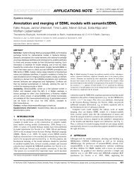
The raw intensity signals generated by this process are known to<br />
be subject to several biases (Aird, et al., 2011; Bravo and Irizarry,<br />
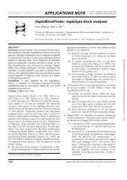
2010; Dohm, et al., 2008; Erlich, et al., 2008) (Figure 1 A, B): 1.<br />
Cross talk: there are significant correlations between different nucleotide<br />
channels; 2. Phasing/Pre-phasing: the signal in one cycle<br />
can spread to the cycles ahead and the cycles after it; 3. Signal<br />
decay: where signal intensities become lower in later sequencing<br />
cycles; 4. Background noise: the signal to noise ratio becomes<br />
lower in later sequencing cycles. A significant challenge in <strong>base</strong><strong>calling</strong><br />
is accounting for these biases.<br />
Existing <strong>base</strong>-<strong>calling</strong> methods can be classified into two major<br />
groups: 1) unsupervised model-<strong>base</strong>d methods that capture the<br />
sequencing-by-synthesis process in a statistical model <strong>of</strong> fluorescence<br />
intensity from which <strong>base</strong>-call probabilities can be extracted<br />
directly (Bravo and Irizarry, 2010; Kao and Song, 2011; Kao, et<br />
Downloaded from http://bioinformatics.oxfordjournals.org/ by guest on February 17, 2014<br />
© The Author(s) 2014. Published by Oxford University Press.<br />
This is an Open Access article distributed under the terms <strong>of</strong> the Creative Commons Attribution License<br />
(http://creativecommons.org/licenses/by/3.0/), which permits unrestricted reuse, distribution, and<br />
reproduction in any medium, provided the original work is properly cited.<br />
1
.<br />
al., 2009; Massingham and Goldman, 2012) and 2) supervised<br />
methods that train a statistical model on a set <strong>of</strong> <strong>base</strong>-calls whereby<br />
Figure 1 Signal properties in the <strong>base</strong>-<strong>calling</strong> problem. (A) Fluorescence intensity measurements from one cluster for fifty sequencing cycles. Crosstalk<br />
and signal decay effects are clearly observed in this data. Background intensity increases as sequencing progresses. (B) The phasing effect demonstrated<br />
on a subset <strong>of</strong> data from panel A. High intensity in the C channel in cycle 32 affects background intensity in the C channel in neighboring cycles.<br />
fluorescence intensity measurements are classified into <strong>base</strong>-calls<br />
(Erlich, et al., 2008; Kircher, et al., 2009). The former methods<br />
have been shown to significantly improve the accuracy <strong>of</strong> Bustard<br />
<strong>base</strong>-calls. These model-<strong>base</strong>d methods aim to capture the sequencing<br />
process described above in a statistical model from<br />
which <strong>base</strong>-call probabilities are usually obtained. While these<br />
probabilistic or machine-learning methods improve the accuracy <strong>of</strong><br />
<strong>base</strong>-calls, they are impractical for use due to their computational<br />
inefficiency, which usually scales quadratically with read length<br />
since most <strong>of</strong> them resort to dynamic programming for model fitting<br />
(Kao and Song, 2011; Kao, et al., 2009; Massingham and<br />
Goldman, 2012).<br />
In this paper, we show that the <strong>base</strong>-<strong>calling</strong> problem can be formulated<br />
as an optimization problem called blind deconvolution.<br />
Based on this observation, we developed <strong>BlindCall</strong> as a method<br />
that treats <strong>base</strong>-<strong>calling</strong> as a blind deconvolution problem (Levin, et<br />
al., 2011; Xu, et al., 2013). We model intensity signals (B) output<br />
by the sequencer as the convolution <strong>of</strong> a latent sparse signal <strong>of</strong><br />
interest X and a convolution kernel k modeling cross-talk and phasing<br />
biases, plus background noise N:<br />
B = k ∗ X + N<br />
The blind deconvolution problem is to recover the latent signal X<br />
given only the observed B. This reduces the <strong>base</strong>-<strong>calling</strong> problem<br />
into solving an inverse problem that admits computationally efficient<br />
solutions. The blind deconvolution problem has been a research<br />
hotspot in recent years (Levin, et al., 2011; Xu, et al., 2013)<br />
and we adapt methods for its solution to the <strong>base</strong>-<strong>calling</strong> problem<br />
(Wang and Yin, 2010).<br />
<strong>BlindCall</strong> was able to provide <strong>base</strong>-calls at comparable accuracy<br />
to state-<strong>of</strong>-the-art probabilistic methods while processing data at<br />
rates ten times or <strong>fast</strong>er in most cases. It scales linearly with read<br />
length and is thus better suited for new long-read sequencing technologies.<br />
Direct blind deconvolution modeling and the <strong>ultra</strong>efficient<br />
processing <strong>base</strong>d on optimization methods presented here<br />
are essential for bioinformatics analysis workflows to cope with<br />
increased <strong>throughput</strong> and read lengths in new sequencing technologies.<br />
2 METHODS<br />
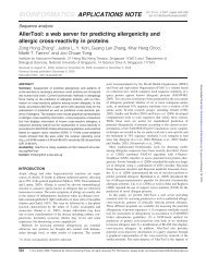
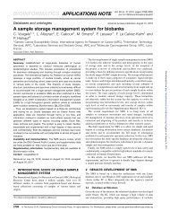
<strong>BlindCall</strong> follows the following architecture (Figure 2A): a training<br />
module uses blind deconvolution (Figure 2B) on a randomly<br />
sampled subset (e.g. 1000 reads) <strong>of</strong> the intensity data to iteratively<br />
estimate the convolution kernel k and produce a deconvolved signal<br />
from which <strong>base</strong>-<strong>calling</strong> is performed. The <strong>base</strong>-<strong>calling</strong> module<br />
then uses the convolution kernel estimated in the training module<br />
to produce a deconvolved output signal for the entire dataset and<br />
call <strong>base</strong>s.<br />
Figure 2. The <strong>BlindCall</strong> architecture. <strong>BlindCall</strong> consists <strong>of</strong> two modules:<br />
(A) the training module uses blind deconvolution (B) to simultaneously<br />
estimate model parameters and produce a deconvolved signal from which<br />
<strong>base</strong>-<strong>calling</strong> is done. The <strong>calling</strong> module uses the parameters estimated in<br />
the training module to produce a deconvolved output signal.<br />
2.1 Blind deconvolution<br />
We solve the Blind Deconvolution problem using an iterative procedure:<br />
a) fixing k and estimating latent signal X using a specific<br />
non-blind deconvolution method <strong>base</strong>d on iterative support detec-<br />
Downloaded from http://bioinformatics.oxfordjournals.org/ by guest on February 17, 2014<br />
2
tion (described below) and then, b) fixing X to estimate convolution<br />
kernel k to correct for cross-talk and phasing effects. We divide<br />
the signal into non-overlapping windows: in each 20-cycle<br />
window we assume an invariant convolution kernel. The discrete<br />
convolution can be written as matrix multiplication B = KX ,<br />
where K is a convolution matrix constructed from the kernel k. A<br />
normalization procedure is used in each iteration to account for<br />
intensity biases across channels.<br />
2.2 Channel intensity normalization<br />
Intensity data for Illumina sequencing show certain biases, specifically,<br />
1) signal strength variation across channels, 2) signal<br />
strength variation across clusters, and 3) signal decay over sequencing<br />
cycles. For accurate <strong>base</strong>-<strong>calling</strong>, these biases must be<br />
addressed through normalization. Traditionally, read normalization<br />
is applied to tackle the second and third problems first, in order to<br />
address the first problem. In our method, we circumvent the read<br />
normalization problem by analyzing the relative intensity ratio <strong>of</strong><br />
successive calls across sequence reads.<br />
After an initial deconvolution in which cross-talk is corrected,<br />
we normalize each channel by scaling the intensities across reads<br />
by the same quantile (95%) in the respective channels and select<br />
the strongest channel after normalization as candidate <strong>base</strong>-calls.<br />
We then select successive candidate calls that are <strong>of</strong> different <strong>base</strong>s<br />
and construct a set <strong>of</strong> linear equations <strong>of</strong> the form x − r x = 0 ,<br />
where<br />
x i k<br />
and<br />
j k<br />
ik<br />
k jk<br />
x are the relative intensity <strong>of</strong> channels in the k-th<br />
relation and r<br />
k<br />
is the observed intensity ratio for the k-th relation.<br />
The set <strong>of</strong> linear equations is then Rx = 0 , where R is a M × 6<br />
matrix, with M being the total number <strong>of</strong> <strong>base</strong>-calls pairs within<br />
consideration. To estimate x we solve a least-squares problem under<br />
the constraint that x 2 =1 . The solution is obtained by solving<br />
an eigenvalue problem since it can be formulated into the Rayleigh<br />
quotient min Rx<br />
2<br />
x = 1<br />
2<br />
, and its solution must satisfy the eigenvalue<br />
equation R t Rx = λx<br />
. Since the number <strong>of</strong> <strong>base</strong>-calls across<br />
channels varies, the solution <strong>of</strong> this optimization problem favors<br />
channels that are called frequently. We normalize the problem<br />
using the number <strong>of</strong> <strong>base</strong>-calls and solve the generalized eigenvalue<br />
problem R Rx = λDx<br />
where D is a diagonal matrix that rec-<br />
t<br />
ords the number <strong>of</strong> <strong>base</strong>-calls in each channel. This formulation<br />
can be interpreted as finding the stable state <strong>of</strong> a normalized nonlinear<br />
diffusion, and is used in normalized cut (Shi and Malik,<br />
2000), Laplacian Eigenmaps (Belkin and Niyogi, 2001), and PageRank<br />
(Page, et al., 1999). The estimated vector x is the relative<br />
intensity <strong>of</strong> each channel and we use it to normalize each channel<br />
in subsequent steps.<br />
2.3 Sparse signal reconstruction through iterative support<br />
detection<br />
To perform <strong>base</strong>-<strong>calling</strong> we need to reconstruct latent sparse signal<br />
X, corresponding only to nucleotide incorporation measurements<br />
2<br />
given a convolution kernel k. A straightforward l optimization<br />
problem to estimate latent signal X minimizes<br />
B − k * X<br />
2<br />
. We<br />
know the latent signal is sparser than the observed signal, so we<br />
add this property as a constraint to the least squares problem and<br />
use an iterative procedure to solve the problem under the sparsity<br />
constraint. This idea is termed iterative support detection (ISD) in<br />
the mathematical community (Wang and Yin, 2010), and can also<br />
be applied to deconvolution problems stemming from image<br />
deblurring applications. In our case, the support (non-zero entries)<br />
detected for latent signal X corresponds exactly to <strong>base</strong>-calls. Assuming<br />
X is the signal taking non-zeros only in the support set<br />
Supp<br />
obtained using our support detection algorithm, we want to find an<br />
X that minimizes<br />
2<br />
2<br />
− ∗ + λ − . This optimization<br />
B k X X X Supp<br />
outputs a corrected signal subject to the support set constraint. The<br />
support detection procedure is critical to the output accuracy – if<br />
the support set is correct, we are close to our solution. At the beginning,<br />
we have no knowledge <strong>of</strong> the support set, since that directly<br />
tells us the answer. To tackle this, we use an increasing series<br />
{ λ<br />
itr}<br />
that puts increasing weight on the second constraint. This<br />
wight is low at first since the support set is not accurate. As we<br />
gradually refine the estimates we increase this weight. In our implementation,<br />
support detection is conducted by incorporating the<br />
channel normalization method discussed in the previous section<br />
and picking the strongest normalized channel.<br />
We provide further mathematical justification as to why this iterative<br />
procedure recovers the clear intensity signals <strong>of</strong> incorporation<br />
events. For reference to the applications in image deblurring<br />
we refer to the convoluted signal B as the blurred signal, and to the<br />
latent signal X, the clear signal.<br />
Observation 1: Assume the clear signal is a non-negative signal<br />
with spikes, the convolution (blur) kernel is non-negative and<br />
k<br />
1<br />
= 1, then the convoluted (blurred) signal is denser than the<br />
latent (clear) signal.<br />
This observation holds for all blurs since the blur spreads the<br />
spikes thus creates more non-zero intensities, so the support set<br />
becomes larger with the blurred signal. This observation hints us to<br />
design an optimization that favors sparse solutions:<br />
2<br />
min B − k * X + λ X ,0 ≤ p ≤ 1<br />
X<br />
The second term is a sparse-inducing penalty. This sparse regularization<br />
problem is well known in wavelet analysis (Mallat,<br />
2009). We also have the following observation:<br />
p<br />
Observation 2: By comparing the l norm (0 ≤ p ≤ 2) <strong>of</strong> the<br />
clear/blurred signal, we discover that the sparse norm penalty favors<br />
the clear signal.<br />
As special cases:<br />
1<br />
• l norm measures the total variation <strong>of</strong> the signal, thus the<br />
blurred signal and clear signal have the same l 1 norm.<br />
• The l 2 norm <strong>of</strong> the blur signal is smaller than that <strong>of</strong> the clear<br />
signal.<br />
• The support set for the blurred signal is larger than the clear<br />
0<br />
signal, therefore it has larger l cost.<br />
The above observations suggest that we use a sparse norm to<br />
penalize the blur signal and make it resemble the clear signal.<br />
0<br />
Thus, we analyze the deconvolution model with an l penalty:<br />
p<br />
2 0<br />
min B − k * X + α X<br />
X<br />
.<br />
By introducing an auxiliary variable and using an exterior penalty<br />
technique, the above minimization problem is equivalent to<br />
solving the following optimization problem:<br />
2 0 2<br />
min B − k * X + α w + λ w − X , λ → +∞<br />
X<br />
.<br />
Downloaded from http://bioinformatics.oxfordjournals.org/ by guest on February 17, 2014<br />
3
.<br />
One strategy to solve the above optimization is the alternating<br />
minimization technique (Wang, et al., 2008) and cast the problem<br />
into two sub-problems: a) fixing X and analyzing the terms containing<br />
w, we have the w sub-problem:<br />
2 α 0<br />
λ<br />
min w − X + w<br />
w<br />
The solution can be found by entry-wise comparison (Mallat,<br />
2009; Xu, et al., 2013) and the result is the so-called hard thresholding:<br />
Supp<br />
⎧<br />
⎪ X<br />
w i<br />
= i<br />
, if | X i<br />
|><br />
α λ<br />
⎨<br />
⎩⎪ 0, otherwise<br />
Then, b) fix w, and analyze the terms containing X, we have<br />
min B − k ∗ X 2 + λ w − X 2<br />
X<br />
This optimization problem has the same form with our deconvolution<br />
model when w = X . In our iterative support detection method,<br />
X<br />
Supp<br />
is obtained by adaptive hard thresholding, where is set<br />
adaptively to select strictly one non-zero element into the support<br />
set by selecting the channel with maximum intensity. Thus, our<br />
iterative support detection method solves an optimization problem<br />
0<br />
with an l penalty favoring sparse signals corresponding to nucleotide<br />
incorporation.<br />
2.4 Convolution kernel estimation<br />
Given latent signal X we use a least-squares method to estimate the<br />
convolution kernel k modeling cross-talk and phasing effects by<br />
solving:<br />
min B − k * X<br />
k<br />
We estimate convolution kernel k in two distinct steps: we use data<br />
from the first four cycles and only model cross-talk in the convolution<br />
kernel and use the blind-deconvolution iterative procedure to<br />
estimate cross-talk effects. We then fix the components <strong>of</strong> the convolution<br />
kernel corresponding to cross-talk effects for the remaining<br />
windows and estimate the components <strong>of</strong> the convolution kernel<br />
corresponding to phasing effects only. We assume the phasing<br />
effect is the same across channels.<br />
2.5 Deriving quality scores from deconvolved signal<br />
We measure the quality <strong>of</strong> a <strong>base</strong>-call by the ratio <strong>of</strong> the intensity<br />
<strong>of</strong> the strongest channel and the sum <strong>of</strong> the two strongest channels<br />
after the deconvolution procedure. This number ranges between<br />
0.5 and 1.0 and is used as the raw quality score. This scheme is<br />
similar to the one in Illumina’s Bustard <strong>base</strong>caller. Like most existing<br />
<strong>base</strong>-callers, we calibrate these raw quality scores by aligning<br />
reads to the reference genome and mapping raw quality scores to<br />
the alignment error rate.<br />
2.6 Validation methods<br />
The following datasets were used to test the accuracy and computational<br />
efficiency <strong>of</strong> <strong>BlindCall</strong> and state-<strong>of</strong>-the-art probabilistic<br />
methods:<br />
Illumina HiSeq 2000 phiX174: 1,926,928 single-end reads <strong>of</strong> 101<br />
cycles from a single tile. Data was sequenced at the University <strong>of</strong><br />
Maryland, College Park and is available for download at<br />
http://cbcb.umd.edu/~hcorrada/secgen.<br />
Ibis Test: 200K single-end reads <strong>of</strong> phiX174 over 51 sequencing<br />
cycles.<br />
2<br />
B. pertussis: 100 tiles <strong>of</strong> 76 cycle single end reads from the coccobacillus<br />
Bordetella pertussis, using the complete genome <strong>of</strong> the<br />
Tohoma I strain as a reference.<br />
AYB phiX174: released with AYB and contains human sequence<br />
with a PhiX174 spike-in.<br />
The last three datasets were downloaded from the AYB authors’<br />
website (http://www.ebi.ac.uk/goldman-srv/AYB/#data).<br />
To calculate accuracy we align the reads <strong>base</strong>d on the phiX174<br />
reference using Bowtie2 (Langmead and Salzberg, 2012) with --<br />
end-to-end and --sensitive settings. Reported error rates<br />
are <strong>base</strong>d on reads with no more than 5 substitution errors, following<br />
the methodology in Massingham and Goldman (2012). We<br />
used SparseAssembler (Ye, et al., 2012) to obtain assemblies from<br />
<strong>base</strong>-calls obtained by each method. To derive assembly statistics,<br />
we sub-sampled 100 datasets from the complete set <strong>of</strong> reads at 5x,<br />
10x and 20x coverage, and perform assemblies on each <strong>of</strong> these.<br />
We report N50 and maximum contig length for each resulting assembly.<br />
Version 1.9.4 <strong>of</strong> the Off-line <strong>base</strong>caller was downloaded from<br />
Illumina to run Bustard. Version 2 <strong>of</strong> AYB was downloaded from<br />
http://www.ebi.ac.uk/goldman-srv/AYB. We ran AYB for 5 iterations<br />
as per its default setting.<br />
3 RESULTS<br />
<strong>BlindCall</strong> is implemented as a set <strong>of</strong> Matlab scripts available at<br />
http://cbcb.umd.edu/~hcorrada/secgen. As an example <strong>of</strong> its computational<br />
efficiency, running <strong>BlindCall</strong> on a single-core Matlab<br />
instance on an Intel i7 3610QM laptop with 2.3-3.3 GHz processor<br />
and 8GB <strong>of</strong> memory, we found that it was able to process 1 million<br />
<strong>base</strong>s per second, or over 85 billion <strong>base</strong>s per CPU day. We note<br />
that a significant portion <strong>of</strong> its running time (50%) is spent on disk<br />
IO to read intensity data and write the <strong>fast</strong>a/<strong>fast</strong>q outputs. To the<br />
best <strong>of</strong> our knowledge, <strong>BlindCall</strong> is one <strong>of</strong> the <strong>fast</strong>est <strong>base</strong>-callers<br />
available at this time, even though it is implemented in a scripting<br />
language. A port <strong>of</strong> this algorithm into a lower-level language<br />
(C/C++) will give further improvements on speed over the current<br />
Matlab version.<br />
We compared the running time <strong>of</strong> <strong>BlindCall</strong> to the state-<strong>of</strong>-the<br />
art probabilistic <strong>base</strong>-caller AYB (Massingham and Goldman,<br />
2012) and the state-<strong>of</strong>-the-art supervised learning method freeIbis<br />
(Renaud, et al., 2013) on a dataset <strong>of</strong> 1.9 million reads from a<br />
PhiX174 run on an Illumina HiSeq 2000 (Table 1). We found that<br />
<strong>BlindCall</strong> was able to process this dataset about 20 times <strong>fast</strong>er<br />
than AYB and 10 times <strong>fast</strong>er than freeIbis while retaining similar<br />
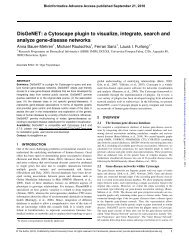
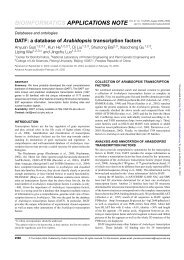
accuracy. A plot <strong>of</strong> per cycle error rate <strong>of</strong> these <strong>base</strong>-callers (Fig.<br />
3) shows that all methods produce significant improvements over<br />
Bustard, especially in later sequencing cycles. We observed a similar<br />
pattern when testing other datasets (Table 2).<br />
Downloaded from http://bioinformatics.oxfordjournals.org/ by guest on February 17, 2014<br />
4
Figure 3. Third party <strong>base</strong>-callers improve Bustard per-cycle error<br />
rate. We plot error rate <strong>of</strong> each <strong>base</strong>-caller per sequencing cycle on the<br />
PhiX174 test data. All three <strong>base</strong>-callers significantly improve accuracy<br />
over Bustard, especially in later cycles. <strong>BlindCall</strong> is able to achieve comparable<br />
accuracy while processing data at a much <strong>fast</strong>er rate.<br />
Table 1. Base-callers accuracy and runtime comparison.<br />
Bustard AYB <strong>BlindCall</strong> Slow <strong>BlindCall</strong> Fast freeIbis<br />
Perfect reads 1446079 1532000 1509451 1508779 1530099<br />
Error rate 0.29% 0.21% 0.23% 0.23% 0.21%<br />
Time (min) 17 217 8/12 4/8 9/126<br />
Assembly Results<br />
N50 Max N50 Max N50 Max N50 Max N50 Max<br />
5x 610 1122 628 1155 629 1164 623 1167 649 1184<br />
10x 3375 3469 3198 3322 3382 3487 3389 3485 3306 3418<br />
20x 4466 4478 4627 4637 4511 4523 4470 4483 4333 4357<br />
Accuracy and run times for Bustard, AYB, freeIbis and <strong>BlindCall</strong> for a dataset <strong>of</strong> 1.9 million reads from a HiSeq 2000 run <strong>of</strong> PhiX174. <strong>BlindCall</strong> Fast corresponds<br />
to non-iterative version <strong>of</strong> the blind-deconvolution method. Running times for <strong>BlindCall</strong> are reported as (processing time / total time), where the total<br />
time includes reading intensity data from disk and writing <strong>base</strong>-calls to disk. For freeIbis, we report the time as (predicting time with single thread/ training<br />
time with 10 threads). <strong>BlindCall</strong> was able to produce <strong>base</strong>-calls <strong>of</strong> comparable accuracy to AYB and freeIbis at significantly <strong>fast</strong>er computational time<br />
(8min/12 min vs. 217 min and 126 min, respectively). It is also <strong>fast</strong>er than Bustard (8 min/12 min vs. 17 min). AYB, freeIbis and <strong>BlindCall</strong> all improve on<br />
Bustard <strong>base</strong>-calls. We also compared assemblies <strong>of</strong> the PhiX174 genome using reads generated by Bustard, <strong>BlindCall</strong>, freeIbis and AYB. The reported<br />
N50s and Max contig lengths are averages over 100 random samples with the corresponding coverage (5x, 10x or 20x). While <strong>BlindCall</strong> is able to process<br />
data at a significantly lower computational cost, the assemblies obtained using <strong>BlindCall</strong> are <strong>of</strong> comparable quality to those obtained using AYB or freeIbis.<br />
from disk and writing <strong>base</strong>-calls to disk.<br />
We also obtained better assemblies, especially at low coverage,<br />
using <strong>BlindCall</strong>, AYB and freeIbis relative to Bustard <strong>base</strong>calls<br />
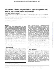
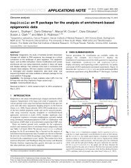
(Table 1). We also found that the calibrated quality values<br />
obtained from <strong>BlindCall</strong> are very accurate (Figure 4).<br />
Table 2. Accuracy comparison.<br />
Ibis Test B. pertussis PhiX174 (AYB)<br />
Perfect<br />
Reads<br />
Error<br />
Rate<br />
Perfect<br />
Reads<br />
Error<br />
Rate<br />
Perfect<br />
Reads<br />
Error<br />
Rate<br />
Bustard 99834 1.45% 1557963 2.01% 24478 0.49%<br />
AYB 133537 0.73% 2304005 1.26% 26878 0.38%<br />
<strong>BlindCall</strong> 110951 1.12% 1902621 1.61% 25144 0.45%<br />
slow<br />
<strong>BlindCall</strong> 105312 1.26% 1856286 1.66% 24740 0.47%<br />
<strong>fast</strong><br />
Time:<br />
slow<strong>fast</strong><br />
0.08/0.3/1<br />
0.11/6/10<br />
0.15/14/22<br />
Downloaded from http://bioinformatics.oxfordjournals.org/ by guest on February 17, 2014<br />
0.08/0.1/1<br />
0.11/3/8<br />
0.15/7/16<br />
Accuracy for Bustard, AYB and <strong>BlindCall</strong> on various datasets. <strong>BlindCall</strong> was<br />
able to produce comparable accuracy to state-<strong>of</strong>-the-art <strong>base</strong>-callers at significantly<br />
<strong>fast</strong>er computational time. All methods improve on Bustard <strong>base</strong>calls.<br />
Run-times for <strong>BlindCall</strong> are reported as (training time/processing time/<br />
total time in minutes) where the total time includes reading intensity data<br />
Figure 4. <strong>BlindCall</strong> produces accurate calibrated quality scores. We<br />
plot observed error rates (on the PHRED scale) for Bustard, AYB and<br />
<strong>BlindCall</strong> as predicted by quality scores and observed <strong>high</strong> correlation<br />
for all <strong>base</strong>-callers.<br />
5
.<br />
We next compared each <strong>base</strong>-<strong>calling</strong> method’s ability to scale<br />
to longer read lengths by calculating running time as a function<br />
<strong>of</strong> read length for the same dataset. Like most probabilistic<br />
model-<strong>base</strong>d <strong>base</strong> callers, AYB resorts to a dynamic programming<br />
strategy with quadratic running time complexity with respect<br />
to the read length. In contrast, <strong>BlindCall</strong> scales linearly<br />
with read length. freeIbis uses supervised learning approach, and<br />
while it also scales linearly with read length, its training time is<br />
much slower than <strong>BlindCall</strong> (even using 10 threads for freeIbis,<br />
compared to a single thread for <strong>BlindCall</strong>). Base-callers <strong>base</strong>d<br />
on the blind deconvolution framework will be able to scale as<br />
sequencers produce longer reads.<br />
methods will be better suited to cope with increased <strong>throughput</strong><br />
and read lengths <strong>of</strong> new sequencing technologies.<br />
ACKNOWLEDGEMENTS<br />
We thank Najib El-Sayed and the University <strong>of</strong> Maryland IBBR<br />
Sequencing core for their assistance with test data, James A.<br />
Yorke and his research group in University <strong>of</strong> Maryland for<br />
insightful discussions, and Gabriel Renaud at Max Planck Institute<br />
for assistance with freeIbis.<br />
This work was partially supported by the National Institute <strong>of</strong><br />
Health [R01HG005220] and [R01HG006102].<br />
Figure 5. Base-<strong>calling</strong> by blind deconvolution is scalable to long read<br />
lengths. We compare the computational time <strong>of</strong> <strong>BlindCall</strong> with a state<strong>of</strong>-the-art<br />
probabilistic <strong>base</strong>-caller AYB, the state-<strong>of</strong>-the-art supervised<br />
learning method freeIbis and Illumina’s Bustard on the PhiX174 dataset<br />
reported in Table 1 as a function <strong>of</strong> the number <strong>of</strong> sequencing cycles.<br />
Since most model-<strong>base</strong>d <strong>base</strong> callers resort to a dynamic programming<br />
solution, running time is quadratic with respect to the read length. In<br />
contrast, <strong>BlindCall</strong> scales linearly with read length. Base-callers <strong>base</strong>d<br />
on the blind deconvolution framework will be able to scale as sequencers<br />
produce longer reads. freeIbis also scales linearly but is much slower<br />
than <strong>BlindCall</strong>.<br />
CONCLUSION<br />
<strong>BlindCall</strong> is a simple and <strong>ultra</strong>-<strong>fast</strong> non-probabilistic <strong>base</strong><strong>calling</strong><br />
method for Illumina <strong>high</strong>-<strong>throughput</strong> sequencing data<br />
<strong>base</strong>d on blind deconvolution. We have shown that it provides<br />
comparable accuracy to probabilistic <strong>base</strong>-<strong>calling</strong> methods while<br />
producing <strong>base</strong>-calls at rates more than ten times <strong>fast</strong>er.<br />
Almost all probabilistic methods solve the <strong>base</strong>-<strong>calling</strong> problem<br />
in a forward way, i.e. by setting a set <strong>of</strong> basis functions and<br />
searching for an optimal path, which <strong>of</strong>ten leads to dynamic<br />
programming solutions. Fitting these statistical methods is computationally<br />
expensive, and will not scale as the increase in sequencing<br />
<strong>throughput</strong> continues. Also, a stationarity assumption<br />
must be made in order to estimate parameters in these probabilistic<br />
methods through a Markov process. In contrast, <strong>BlindCall</strong><br />
models <strong>base</strong>-<strong>calling</strong> as an inverse problem <strong>of</strong> blind deconvolution,<br />
which requires no probabilistic assumptions <strong>of</strong> the sequencing<br />
process.<br />
As steady progress has been made to improve the accuracy <strong>of</strong><br />
probabilistic methods, we expect that similar progress will be<br />
made on non-probabilistic methods <strong>base</strong>d on the blind deconvolution<br />
methods described in this paper. Furthermore, these<br />
REFERENCES<br />
Aird, D., et al. (2011) Analyzing and minimizing PCR<br />
amplification bias in Illumina sequencing libraries., Genome<br />
biology, 12, R18.<br />
Alkan, C., Sajjadian, S. and Eichler, E.E. (2011) Limitations <strong>of</strong><br />
next-generation genome sequence assembly, Nature Methods, 8,<br />
61-65.<br />
Belkin, M. and Niyogi, P. (2001) Laplacian Eigenmaps and<br />
Spectral Techniques for Embedding and Clustering, Advances in<br />
neural information processing systems, 14, 585-591.<br />
Bentley, D.R., et al. (2008) Accurate whole human genome<br />
sequencing using reversible terminator chemistry, Nature, 456,<br />
53-59.<br />
Bravo, H.C. and Irizarry, R.a. (2010) Model-<strong>base</strong>d quality<br />
assessment and <strong>base</strong>-<strong>calling</strong> for second-generation sequencing<br />
data., Biometrics, 66, 665-674.<br />
Dohm, J.C., et al. (2008) Substantial biases in <strong>ultra</strong>-short read<br />
data sets from <strong>high</strong>-<strong>throughput</strong> DNA sequencing., Nucleic acids<br />
research, 36, e105.<br />
Erlich, Y., et al. (2008) Alta-Cyclic: a self-optimizing <strong>base</strong><br />
caller for next-generation sequencing, Nature Methods, 5, 679-<br />
682.<br />
Illumina (2013) HiSeq Systems Comparison.<br />
Kao, W.-C. and Song, Y.S. (2011) naiveBayesCall: an efficient<br />
model-<strong>base</strong>d <strong>base</strong>-<strong>calling</strong> algorithm for <strong>high</strong>-<strong>throughput</strong><br />
sequencing., Journal <strong>of</strong> computational biology : a journal <strong>of</strong><br />
computational molecular cell biology, 18, 365-377.<br />
Kao, W.-C., Stevens, K. and Song, Y.S. (2009) BayesCall: A<br />
model-<strong>base</strong>d <strong>base</strong>-<strong>calling</strong> algorithm for <strong>high</strong>-<strong>throughput</strong> shortread<br />
sequencing., Genome research, 19, 1884-1895.<br />
Kircher, M., Stenzel, U. and Kelso, J. (2009) Improved <strong>base</strong><br />
<strong>calling</strong> for the Illumina Genome Analyzer using machine<br />
learning strategies., Genome biology, 10, R83.<br />
Langmead, B. and Salzberg, S.L. (2012) Fast gapped-read<br />
alignment with Bowtie 2, Nature Methods, 9, 357-U354.<br />
Levin, A., et al. (2011) Understanding Blind Deconvolution<br />
Algorithms, IEEE Transactions on Pattern Analysis and<br />
Machine Intelligence, 33, 2354-2367.<br />
Mallat, S.G. (2009) A wavelet tour <strong>of</strong> signal processing : the<br />
sparse way. Elsevier/Academic Press, Amsterdam ; Boston.<br />
Downloaded from http://bioinformatics.oxfordjournals.org/ by guest on February 17, 2014<br />
6
Massingham, T. and Goldman, N. (2012) All Your Base: a <strong>fast</strong><br />
and accurate probabilistic approach to <strong>base</strong> <strong>calling</strong>., Genome<br />
biology, 13, R13.<br />
Page, L., et al. (1999) The PageRank Citation Ranking:<br />
Bringing Order to the Web. Stanford InfoLab.<br />
Renaud, G., et al. (2013) freeIbis: an efficient <strong>base</strong>caller with<br />
calibrated quality scores for Illumina sequencers,<br />
<strong>Bioinformatics</strong>, 29, 1208-1209.<br />
Shi, J.B. and Malik, J. (2000) Normalized cuts and image<br />
segmentation, IEEE Transactions on Pattern Analysis and<br />
Machine Intelligence, 22, 888-905.<br />
Wang, Y. and Yin, W. (2010) Sparse Signal Reconstruction via<br />
Iterative Support Detection, SIAM Journal on Imaging Sciences,<br />
3, 462-491.<br />
Wang, Y.L., et al. (2008) A New Alternating Minimization<br />
Algorithm for Total Variation Image Reconstruction, SIAM<br />
Journal on Imaging Sciences, 1, 248-272.<br />
Xu, L., Zheng, S. and Jia, J. (2013) Unnatural L 0 Sparse<br />
Representation for Natural Image Deblurring, IEEE Conference<br />
on Computer Vision and Pattern Recognition (CVPR).<br />
Ye, C., et al. (2012) Exploiting sparseness in de novo genome<br />
assembly, BMC <strong>Bioinformatics</strong>, 13 Suppl 6, S1.<br />
Downloaded from http://bioinformatics.oxfordjournals.org/ by guest on February 17, 2014<br />
7