Input-output theory of the unconventional photon blockade

PHYSICAL REVIEW A 88, 033836 (2013)
Input-output theory of the unconventional photon blockade
H. Flayac and V. Savona
Institute of Theoretical Physics, École Polytechnique Fédérale de Lausanne EPFL, CH-1015 Lausanne, Switzerland
(Received 11 July 2013; published 23 September 2013)
We study the unconventional photon blockade, recently proposed for a coupled-cavity system, in the presence of
input and output quantum fields. Mixing of the input or output channels still allows strong photon antibunching
of the output field, but for optimal values of the system parameters that differ substantially from those that
maximize antibunching of the intracavity field. This result shows that the specific input-output geometry in
a photonic system determines the optimal design in view of a single-photon device operation. We provide a
compact analytical formula that allows finding the optimal parameters for each specific system geometry.
DOI: 10.1103/PhysRevA.88.033836
PACS number(s): 42.50.Pq, 42.50.Ct, 03.65.−w, 71.36.+c
I. INTRODUCTION
The generation of single photons is a crucial requirement
in information and communication technology [1]. A singlephoton
source typically relies on a system able of producing
sub-Poissonian light when driven by a classical light field.
This mechanism requires a strong optical nonlinearity, such
that the optical response to one photon can be modulated by
the presence or absence of a single photon in the system, the
so-called photon blockade. Combined with the requirement
of miniaturization for integrability and scalability purposes,
a strong nonlinearity is typically achieved by increasing the
time duration of the interaction between light and a small
nonlinear system (e.g., a two-level optical transition), by means
of a resonant optical cavity. This basic paradigm, from which
the research area called cavity quantum electrodynamics [2]
stems, was proposed long ago [3], and has been meanwhile
experimentally demonstrated in atomic [4], semiconductor
[5–7], and superconducting [8] hybrid systems, while theoretical
proposals have been formulated for optomechanical
systems [9–12]. Yet, to achieve a sizable photon blockade
in these systems, the energy scale characterizing the optical
nonlinearity must be large, i.e., it must exceed the optical
losses, thus posing a severe technological challenge.
Recently, a paradigm for the generation of sub-Poissonian
light was proposed [13]. Such unconventional photon blockade
(UPB) [14] differs from the conventional mechanism in that
the blockade is enforced by quantum interference between
multiple excitation pathways [15], rather than by an effective
photon-photon repulsion induced by the strong nonlinearity.
The UPB mechanism occurs in a system of two coupled
cavities, where the linear coupling strength is the dominant
energy scale, while a very weak third-order nonlinearity
characterizes the two resonators. UPB displays a strong
resonant behavior, as a function of the two modes energies and
the coupling strength. It is essentially thanks to this resonant
character that the effect of a very weak nonlinearity can be
amplified almost at will, to produce photon blockade. UPB
holds great promise as an alternative paradigm in view of an
integrated and scalable technology for single-photon generation
[16]. Several possible implementations of this effect are
currently being considered, for example, in polaritonic [17],
optomechanical [18,19], or photonic crystal systems [16,20].
Each of these possible implementations is based on a system
design that includes a specific scheme of input and output
channels. In the original proposal, the basic UPB mechanism
occurs only for the intracavity field of one of the two cavities.
In a realistic implementation, each of the two cavities couples
predominantly to a different input and output channel, but
unavoidably some mixing between the two input or the two
output channels must be expected. An example could be that
of a system based on a photonic crystal slab [16], in which the
mixing is simply produced by proximity between the cavities
and the input-output channels. Given the interferential nature
of UPB, a very natural expectation is that such a mixing may
affect the mutual phase relation between fields, ultimately
suppressing the antibunching [17,20].
Here, we study the UPB mechanism by modeling quantum
input and output channels with arbitrary degree of mixing.
We compute the two-photon correlation function at zero
delay, both numerically by fully solving the system master
equations, and analytically in the limit of weak driving field.
We demonstrate that, contrarily to common expectations, an
optimal condition for UPB still exists for arbitrary degree
of mixing, but it occurs for system parameters (particularly
the resonant frequencies of the two cavities) that differ
considerably from those derived for the intracavity field [15].
Our result thus shows that each system design of the inputoutput
channels determines different optimal parameters for
UPB. These parameters must then be modeled appropriately
before fabrication, as they determine the optimal design. In
the Appendix section, we provide a compact analytical tool
that allows us to easily link the input-output mixing rates to
the optimal design of the two cavities.
II. INTRACAVITY FIELDS
In cavity quantum electrodynamics, several specific systems
display nonlinear optical properties that can be mapped,
under appropriate conditions, onto the simple model of an
oscillator with a third-order nonlinearity. We recall here the
three most common cases; first, an optical cavity embedding
a Kerr optical medium [21]; second, an optical cavity whose
resonant mode is coupled to the optical transition of a two-level
system, well described by the Jaynes-Cummings model which
has widespread applications to atomic [4], semiconductor [7],
and superconducting systems [22] (in this case, the equivalence
holds only in the limit of large detuning between the cavity
mode and the two-level transition, compared to the coupling
strength [23,24]); third, an optomechanical system in which the
1050-2947/2013/88(3)/033836(7) 033836-1
©2013 American Physical Society

H. FLAYAC AND V. SAVONA PHYSICAL REVIEW A 88, 033836 (2013)
optical density inside the cavity is coupled to the displacement
of a mechanical oscillator [11,25]. Given this broad range of
currently investigated systems, it is therefore interesting to
study quantum optical effects using the model of an oscillator
with third-order nonlinearity.
Here, we consider the system of two coupled single-mode
cavities, described respectively by Bose operators â 1,2 and â † 1,2 ,
as originally studied in Ref. [13]. Both modes are characterized
by a weak third-order nonlinearity of strength U and are
driven by continuous-wave fields having the same frequency
ω L and distinct amplitudes F 1,2 . In the frame rotating at ω L ,
the intracavity Hamiltonian reads as
H = ∑ [
Ej â † j âj + Uâ †2
j â2 j + F j â † j + F j ∗ ]
âj
j=1,2
− J (â
1â2 † + â 2â1), † (1)
where E 1,2 are the mode energies expressed with respect to ω L .
The system dynamics is governed by the following quantum
master equation for the density matrix ˆρ:
i d ˆρ = [H, ˆρ] + L (rad) + L (pd) , (2)
dt
where
L (rad) = i ∑
Ɣ j (2â j ˆρâ † j
2
−{↠j âj , ˆρ}), (3)
j=1,2
L (pd) = i ∑
Ɣ (pd)
j
(2â † j
2
âj ˆρâ † j âj −{â † j âj â † j âj , ˆρ}) (4)
j=1,2
are Lindblad superoperators modeling, in the Markov limit,
respectively radiative losses at rates Ɣ 1,2 and pure dephasing
processes at rates Ɣ (pd)
1,2
. Following, we will solve numerically
Eq. (2) in the stationary limit d ˆρ/dt = 0, within a truncated
Hilbert space [13].
III. INPUT-OUTPUT FIELDS
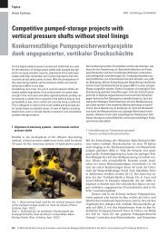
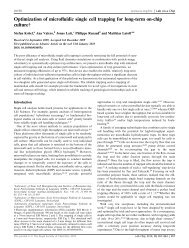
We consider input and output lines as sketched in Fig. 1(a).
We assume two semi-infinite waveguides L b and L c evanescently
coupled to the cavities, in the wake of the proposal
of Ref. [16]. Each waveguide acts simultaneously as an
input and an output channel for the two-cavity system. The
corresponding Bose operators for the input and output modes
are denoted as ˆb in , ˆb out , ĉ in , and ĉ out . The evanescent coupling
of cavities 1 and 2 to waveguides L b and L c is quantified by
the rates γ b,1,2 and γ c,1,2 , respectively. The coherent driving
field is conveyed through the waveguide L b , while the device
output is collected from the L c channel.
According to the input-output formalism of Collett and
Gardiner [26,27], the input, output, and intracavity fields are
linked through the boundary condition
ˆb out(t) (†) = ˆb in (†) + √ γ b,1 â (†)
1
+ √ γ b,2 â (†)
2 , (5)
ĉ out(t) (†) = ĉ in (†) + √ γ c,1 â (†)
1
+ √ γ c,2 â (†)
2 . (6)
The rates γ b,1,2 and γ c,1,2 contribute, together with the intrinsic
loss rate κ 1,2 of each cavity, to the total loss rates of the two
cavity modes, i.e., κ 1,2 + γ b,1,2 + γ c,1,2 = Ɣ 1,2 . All these loss
rates depend on the specific system type and cavity design.
FIG. 1. (Color online) (a) Sketch of the system. Two coupled
cavities are evanescently linked to two semi-infinite waveguides
L b and L c . The blue and red double arrows denote input-output
couplings. The inset shows the energy levels and associated detunings.
Lower panels: log 10 [g out(0)] (2) as a function of E 1 and E 2 for γ 1 = 0.4Ɣ,
(b) γ 2 = 0, and (c) γ 2 = 0.025γ 1 . The other parameters are κ 1,2 =
Ɣ − 2γ 1,2 , U = 0.012/Ɣ, J = 0.5/Ɣ,andF = 0.01/Ɣ. The white
cross marks the location of the global minimum of panel (b), while
the circles indicate the two local minima, and the arrows highlight
their displacement as γ 2 is increased.
Here, in order to comply to the assumption made in Ref. [13],
we set Ɣ 1 = Ɣ 2 = Ɣ. Notice that this assumption generally
leads to different intrinsic loss rates κ 1,2 for the two cavities.
The extension to more general assumptions is, however,
straightforward. Additionally, we shall consider a system that
is symmetric with respect to the input-output guides imposing
γ 1,2 = γ b,1,2 = γ c,1,2 . The ideal case described of Ref. [13]
is then recovered by setting γ 2 = 0. A finite value of γ 2
expresses instead the fact that any output observable includes
contributions from both intracavity fields. This is unavoidable
in most experimental setups, where both the coupling between
cavities 1 and 2 and the coupling to input-output lines are
realized through spatial proximity, as suggested by the sketch
in Fig. 1(a).
For an arbitrary state of the input modes, correlations of
the output fields would depend on cross correlations between
the input and intracavity fields, which in turn would require
to model the input fields together with the system dynamics.
However, if we assume only classical driving fields added to
the quantum vacuum of the input-output channels, then all
normally ordered cross correlations between intracavity and
input modes vanish, and correlations in the output channels
can be expressed as functions of intracavity correlations
only. Within this assumption, the average number of photons
collected through L c reads as
N out =〈ĉ outĉ † out 〉
= γ 1 〈â 1â1〉+γ † 2 〈â 2â2〉+2 † √ γ 1 γ 2 〈â
1â2 † + â 2â1〉. † (7)
033836-2

INPUT-OUTPUT THEORY OF THE UNCONVENTIONAL ... PHYSICAL REVIEW A 88, 033836 (2013)
g (2)
out (0)
E 2
/Γ
1
0.8
0.6
0.4
-1
1
0.8
0.6
0.4
0.2
0.2
2
3
(a)
(b)
0
0
2
0 0.1 0.2 0 0.1 0.2 0 0.5 1 0 0.2 0.4 0.6
γ /γ γ 2 1
2
/γ 1
γ /γ γ /γ 2 1
2 1
0
0
1.5
(e) (f) (g) (h)
-2
-4
g (2)
out (0)
F/Γ
x10 -2 x10 -2
6
(c) 7 (d)
5
4
3
1
6
5
4
8
6
4
-2
0.5 1 1.5
E 1
/Γ
-6
2 4 6
E 1
/Γ
0.5
0 0.5 1
γ 2
/γ 1
2
0 0.2 0.4 0.6
γ 2
/γ 1
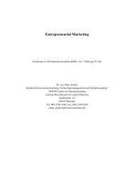
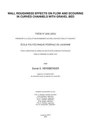
FIG. 2. (Color online) Steady-state solutions of Eq. (2). (a)g out(0) (2) as a function of γ 2 /γ 1 at constant detunings E 1,2 =±Ɣ/2 √ 3 [white
cross in Fig. 1(c)]. (b) Same as (a), when also accounting for the input mixing Eq. (10). These values do not depend significantly on γ 1 .(c),
(d) Same as, respectively, (a) and (b), but tracking min[g out(0)] (2) as a function of E 1 and E 2 for each value of the abscissa. Red squares, purple
disks, blue triangles, and light blue diamonds correspond to γ 1 = 0.2, 0.3, 0.4, and 0.5, respectively. The corresponding displacement on the
(E 1 ,E 2 ) plane is shown in panels (e) and (f), respectively. This displacement is essentially independent of γ 1 . (g), (h) Pump amplitude required
to give a constant occupation N out = 10 −3 for the data in panels (c) and (d), respectively.
Similarly, the second-order correlation function of the output
field at zero delay is given by
g out(0) (2) = 〈ĉ† outĉ outĉ † out ĉ out 〉
Nout
2 (8)
= ∑
j,k,l,m=1,2
√ 〈â † j γj γ k γ l γ ↠kâlâ m 〉
m . (9)
N 2 out
If the driving fields are delivered through the two waveguides,
then the same mixing weights must hold given the
system symmetry, namely,
√
γ1,2
F 1,2 = F, (10)
γ 1 + γ 2
so that |F | 2 =|F 1 | 2 +|F 2 | 2 .
IV. RESULTS
The antibunching of the intracavity field is maximized for
optimal values [15]
E 1,2 ≃±Ɣ/2 √ 3, (11)
U ≃ 2Ɣ 3 /3J 2√ 3. (12)
Here, we set U to its optimal value (12), and let the detunings
E 1 and E 2 vary. Figure 1(a) shows the computed value of
log 10 [g out(0)], (2) as a function of E 1 and E 2 , in the case γ 2 = 0,
namely, without mixing. The result reproduces exactly that
for the intracavity field in Ref. [13]. When instead a finite
value γ 2 = 0.025γ 1 is set, the optimal antibunching moves
to different values of E 1 and E 2 , and the original minimum
splits into two distinct minima. Indeed, if the optimal values
(11) and (12) are set, the value of g (2)
out(0) rapidly increases
as a function of γ 2 /γ 1 , both when assuming output mixing
only [Fig. 2(a)] and if a corresponding input mixing (10) is
introduced [Fig. 2(b)]. These results suggest that the optimal
values of E 1 and E 2 must be found independently for each
value of γ 2 . We note that the absolute value of γ 1 has practically
no influence on this behavior which is solely determined by
the ratio γ 2 /γ 1 .
To illustrate how the optimal values of E 1 and E 2 depend
on the mixing, we plot on the (E 1 , E 2 ) plane the position
of the minimum labeled m 1 in Fig. 1(c), forγ 2 /γ 1 uniformly
increasing from 0 to 0.5, both in the case of output mixing
only [Fig. 2(e)] and including input mixing [Fig. 2(f)]. Again,
these values scarcely depend on the absolute value of γ 1 .
Correspondingly, Figs. 2(c) and 2(d) show the value of g (2)
out(0)
computed at increasing γ 2 /γ 1 , while tracking the optimal
values of E 1 and E 2 as a function of this parameter. Here,
different symbols denote different values of γ 1 , showing that
this parameter affects the actual value of the two-photon
correlation. For these plots, the overall pump amplitude F
was also adjusted for each value of γ 2 /γ 1 in order to keep
the average photon occupation in the output mode constant
N out = 10 −3 . The corresponding values of F are plotted in
Figs. 2(g) and 2(h), respectively. These data show that the
unconventional antibunching can indeed be preserved, or even
slightly improved, when tuning the optimal values of E 1 and
E 2 to the ratio of output coupling rates γ 2 /γ 1 characterizing
the specific system under investigation.
033836-3

H. FLAYAC AND V. SAVONA PHYSICAL REVIEW A 88, 033836 (2013)
g (2)
out (0)
g (2)
out (0)
10 0
10 -1
(a)
10 -2
-2 0 2 4 6 8
Δ /Γ 12
10 0 (c)
10 -1
10 -2
0 0.2 0.4 0.6
γ /γ 2 1
E 1
/Γ
E 2
/Γ
8 3
6 2
4 1
2
0
-2
-4
0
-1
-2
-3
F/Γ
(b)
-2 0 2 4 6 8
Δ /Γ 12
1.5
-4
(d)
0 1 2 3 4
E /Γ 1
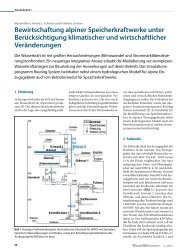
FIG. 3. (Color online) (a) Minimal value of g out(0) (2) as a function of
the detuning 12 , obtained by varying E 1 . (b) Corresponding optimal
value of E 1 . Inset: value of F required to give a constant occupation
N out = 10 −3 . For both plots, γ 1 = 0.2Ɣ (red squares), 0.3Ɣ (purple
disks), and 0.4Ɣ (blue triangles). (c) Impact of the pure dephasing
on min[g out(0)] (2) for Ɣ (pd) = 0 (red squares), 0.01U (purple disks),
and 0.1U (blue triangles). (d) Corresponding points on the (E 1 ,E 2 )
plane. Inset: value of F required to impose a constant occupation
N out = 10 −3 .
When considering a given engineered sample, the detuning
between the two cavities 12 = E 1 − E 2 is generally determined
by the specific sample design and fabrication. It is therefore
relevant, in view of an experiment, to study the optimal
value of the detuning E 1 for each given value 12 . The corresponding
results (accounting for the mixed input) are shown
in Figs. 3(a) and 3(b). Figure 3(a) shows the optimal value
of g (2)
out(0) computed as a function of 12 for three different
values of γ 2 , while Fig. 3(b) shows the corresponding optimal
value of E 1 and the pump amplitude (inset) required to have
N out = 10 −3 . As soon as the output fields are mixed we see that
optimal antibunching requires 1,2 > 0, differently from the
ideal case [13,15] where 12 ≃ 0. In the cases where γ 2 ≠ 0,
two distinct minima in g (2)
out appear, consistently with Fig. 1(c).
Finally, we have analyzed in Figs. 3(c) and 3(d) the impact
of pure dephasing, as introduced in Eq. (4), for three values of
Ɣ (pd) = Ɣ (pd)
1
= Ɣ (pd)
2
. While the optimal values of E 1 and E 2
are only slightly affected [Fig. 3(d)], the corresponding optimal
value of min[g out(0)] (2) increases significantly [Fig. 3(c)], as
expected for the unconventional mechanism which strongly
relies on quantum interference. In particular, antibunching
starts being suppressed as soon as the pure dephasing rate
becomes comparable to the nonlinear energy U. Thisisagain
expected, as the destructive quantum interference between
different excitation pathways leading to the two-photon state is
enforced by a nonlinear energy shift of magnitude U. It can be
concluded that the sensitivity to pure dephasing is not dramatically
modified by mixing in the input or in the output channels.
2
1
F/Γ
UPB relies on the fact that, thanks to destructive quantum
interference between multiple excitation pathways leading to
the state with two photons in the first cavity, the amplitude
of this particular number state in the stationary state of
the system vanishes under appropriate choice of the system
parameters. Then, in the limit of vanishing pump amplitude
F , the probability of having N 1 > 2 is negligible and g (2)
out(0)
actually vanishes as a result. In the presence of output mixing,
however, Eqs. (5) and (6) show that an analogous canceling
of the two-photon amplitude in the output field now requires
suppressing the two-photon occupation of the mode associated
to the linear superposition √ γ 1 â 1 + √ γ 2 â 2 . This is made
possible by a similar quantum interference scheme as in
the ideal case where, however, optimal conditions occur for
different values of the detunings E 1 and E 2 . This is ultimately
the reason why output mixing does not actually suppress
antibunching but rather moves it to a different optimal point in
parameter space. More insight on this result can be obtained
by carrying out an analysis to leading order in F , similar to the
one presented for the ideal case in Ref. [15]. This leads to a
compact analytical expression for g (2)
out(0) in the limit F → 0,
derived in the Appendix, that can be easily adopted to optimize
the parameters E 1 and E 2 in each specific case.
The main indication coming from this study is that, in any
attempt to experimentally design a coupled-cavity system for
the detection of unconventional photon blockade, the input and
output mixing must be accurately modeled before fabrication,
in order to assess the corresponding optimal detuning 12 =
E 1 − E 2 between the two cavities.
V. CONCLUSION
In summary, we have studied the unconventional photon
blockade in the context of an input-output theory of the
open quantum system, in order to assess how unavoidable
mixing between the two input or the two output channels
affects the photon antibunching. Our findings clearly show
that the photon antibunching is not suppressed but rather just
displaced in a different region of the system’s parameter space.
Unconventional photon blockade was recently proposed as a
very effective mechanism to produce a strongly sub-Poissonian
photon field in the presence of arbitrarily weak nonlinearities.
This mechanism holds great promise in view of the realization
of integrated single-photon sources, that could operate even by
only relying on the very weak background third-order nonlinearity
of the dielectric material [16], and could be the mechanism
of choice to observe quantum effects in hybrid systems,
such as, i.e., optomechanical systems [18,19], where strong
single-photon nonlinearities are far from being achieved.
It should be observed that, to operate as an on-demand
single-photon source, a system displaying the unconventional
photon blockade would additionally require pulsed operation,
for which the unconventional blockade mechanism is subject
to some restrictions as discussed by Bamba et al. [17]. In
particular, in order for antibunching to occur in the pulsed
regime, the bandwidth of the pump pulse must be smaller than
the cavity loss rate Ɣ, while its time duration must be shorter
than the time scale of the quantum correlations, set by J −1 .
These two conditions are barely met for the typical regime J>
Ɣ, in which the unconventional blockade occurs. A possible
033836-4

INPUT-OUTPUT THEORY OF THE UNCONVENTIONAL ... PHYSICAL REVIEW A 88, 033836 (2013)
way to overcome this limitation might be to filter the output
either in frequency or in time, a task for which the present
input-output theory is the appropriate tool. Spectral filtering in
particular has been shown to enhance photonic antibunching
of the conventional type [28]. Alternatively, an appropriate
shaping of the pump pulse might also improve single-photon
operation. These ideas, however, require verification through a
time-resolved analysis of the unconventional photon blockade,
which will be the object of future work.
Our study shows that, in order to produce the optimal
conditions for the unconventional blockade, the systemspecific
input-output relations play a crucial role, affecting
dramatically the optimal system design. The present result
clearly indicates what are the optimal system parameters and
provides a tool for their evaluation, that can be easily adopted
in the several contexts, ranging from photonic crystal [16,20]
to optomechanical [18,19] or polaritonic [13,15,17] systems,
in which an experimental demonstration of the unconventional
photon blockade is currently being sought.
ACKNOWLEDGMENTS
We are grateful to D. Gerace and S. Savasta for fruitful
discussions. Our work was supported by NCCR Quantum
Photonics (NCCR QP), research instrument of the Swiss
National Science Foundation (SNSF).
APPENDIX: WEAK PUMP LIMIT
In this section, we derive analytical expressions for the
number of intracavity photons and the zero-delay two-photon
correlation function, in the limit of vanishing driving field.
We start from the Hamiltonian (1) and expand the intracavity
field wave function on a Fock-state basis, truncated to the
two-photon manifold as allowed by the assumption of weak
driving field
|ψ〉 =C 00 |00〉+C 10 |10〉+C 01 |01〉
+ C 11 |11〉+C 20 |20〉+C 02 |02〉. (A1)
Here, |jk〉=|j〉⊗|k〉 denotes a Fock state with j photons in
the first cavity and k photons in the second one. The steady
state is found from the stationary solution of the nonlinear
Schrödinger equation H ˜ |ψ〉 =i¯h∂ t |ψ〉 written for the non-
Hermitian Hamiltonian
˜ H = H − iƔ 2
∑
j=1,2
â † j âj
(A2)
with the further assumption Ɣ 1,2 = Ɣ. We assume equal
coupling to the two input-output channels, namely, γ b,1,2 =
γ c,1,2 = γ 1,2 and obtain the following coupled set of equations
for the coefficients C jk :
0 = F 1 C 10 + F 2 C 01 , (A3)
0 = F 1 C 02 + F 2
√
2C11 , (A4)
0 = F 2 C 02 + F 1
√
2C11 , (A5)
0 = F 1 C 00 + Ẽ 1 C 10 − JC 01 + F 1
√
2C20 + F 2 C 11 , (A6)
0 = F 2 C 00 + Ẽ 2 C 01 − JC 10 + F 2
√
2C02 + F 1 C 11 , (A7)
0 = F 1
√
2C10 + 2(Ẽ 1 + U 1 )C 20 − J √ 2C 11 , (A8)
0 = F 2
√
2C01 + 2(Ẽ 2 + U 2 )C 02 − J √ 2C 11 , (A9)
0 = F 2 C 10 + F 1 C 01 − J √ 2(C 20 + C 02 ) + (Ẽ 1 + Ẽ 2 )C 11 ,
(A10)
where Ẽ j = E j − iƔ/2. Here, the pump amplitudes are
expressed as F j = √ ζ j F where ζ 1,2 = γ 1,2 /(γ 1 + γ 2 ). To
leading order, the coefficients C jk depend on the driving
field amplitude as C jk ∝ F j+k . Hence, we can eliminate
the underlined terms in Eqs. (A6) and (A7), as they are of
subleading order in F . By further imposing the normalization
condition C 00 = 1, straightforward algebra leads to the
following solutions:
√
C 10 = F Ẽ2 γ1 + J √ γ 2
,
J 2 − Ẽ 1 Ẽ 2
(A11)
√
C 01 = F Ẽ1 γ2 + J √ γ 1
,
J 2 − Ẽ 1 Ẽ 2
(A12)
C 20 = F 2 [Ẽ3
2
+ Ẽ 2 2 (Ẽ 1 + U) + UJ 2] γ 1 + J 2 (Ẽ 1 + Ẽ 2 + U)γ 2 + 2J √ γ 1 γ 2 (Ẽ 1 + Ẽ 2 )(Ẽ 2 + U)
√
2(Ẽ1 Ẽ 2 − J 2 ) { Ẽ 2 1 (Ẽ 2 + U) + Ẽ 1 [(Ẽ 2 + U) 2 − J 2 ] + Ẽ 2 2 U + J 2 (Ẽ 2 − 2U) } , (A13)
C 02 = F 2 [Ẽ3
1
+ Ẽ 2 1 (Ẽ 2 + U) + UJ 2] γ 2 + J 2 (Ẽ 1 + Ẽ 2 + U)γ 1 + 2J √ γ 1 γ 2 (Ẽ 1 + Ẽ 2 )(Ẽ 1 + U)
√
2(Ẽ1 Ẽ 2 − J 2 ) { Ẽ 2 2 (Ẽ 1 + U) + Ẽ 2 [(Ẽ 1 + U) 2 − J 2 ] + Ẽ 2 1 U + J 2 (Ẽ 1 − 2U) } , (A14)
C 11 = F 2 J (Ẽ 1 + Ẽ 2 + U)[(Ẽ 2 + U)γ 1 + J (Ẽ 1 + U)γ 2 ]
(Ẽ 1 Ẽ 2 − J 2 ) [ Ẽ1 2(Ẽ 2 + U) + Ẽ2 2(Ẽ 1 + U) − J 2 (Ẽ 1 + Ẽ 2 − 2U) ],
√ [
+ F 2 γ1 γ 2 (Ẽ1 + Ẽ 2 )(Ẽ 1 Ẽ 2 + J 2 + U 2 ) + U ( Ẽ1 2 + ) Ẽ2 2 + 2UẼ1 Ẽ 2 + 2UJ 2]
(Ẽ 1 Ẽ 2 − J 2 ) [ Ẽ1 2(Ẽ 2 + U) + Ẽ2 2(Ẽ 1 + U) − J 2 (Ẽ 1 + Ẽ 2 − 2U) ] , (A15)
033836-5

H. FLAYAC AND V. SAVONA PHYSICAL REVIEW A 88, 033836 (2013)
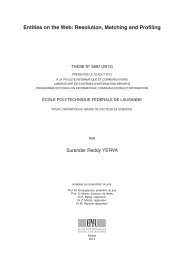
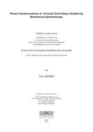
FIG. 4. (Color online) Comparison of the numerical (upper panels) and analytical (lower panels) values of log 10 [g (2)
out(0)], as a function of
E 1 and E 2 ,atfixedγ 1 = 0.4Ɣ,forγ 2 taking values from γ 2 = 0toγ 2 = 0.1γ 1 by steps of 0.02γ 1 from left to right. Here, F = 10 −2 /Ɣand the
other parameters are the same as for Fig. 1.
where we further assumed U 1,2 = U. We then construct the system density matrix from ρ =|ψ〉〈ψ|. By combining this result
with the expressions for the input-output field operators, we obtain the following compact expression for the average photon
occupation in the output field of the first cavity:
N out =〈c outc † out 〉=Tr(c outc † out ρ) =
∣ F (Ẽ √
2 γ1 + J √ γ 2 ) √ √
γ 1 + (Ẽ 1 γ2 + J √ γ 1 ) √ ∣
γ 2 ∣∣∣
2
. (A16)
J 2 − Ẽ 1 Ẽ 2
The second-order correlation function at zero delay of the output field can be expressed in a compact form as a function of the
coefficients C jk as
g out(0) (2) = Tr(c† outc outc † out c out ρ)
Nout
2 ≃ |γ 1C 20 + γ 2 C 02 | 2 +|γ 1 C 20 + √ γ 1 γ 2 C 11 | 2 +|γ 2 C 02 + √ γ 1 γ 2 C 11 | 2
| √ γ 1 C 10 + √ γ 2 C 01 | 4 . (A17)
We compare in Fig. 4 the analytical expression (8) (see lower
panels) to direct numerical solutions of the density matrix
dynamics from Eq. (2) (see upper panels). We get a perfect
agreement between the two for weak pump intensities.
Finally, we show that perfect output antibunching, namely
g out(0) (2) = 0, can not be obtained, differently from the intracavity
field case. In particular, in order to make the numerator of
expression (A17) vanish, one would need
C 02 =− γ 1
C 20 ,
(A18)
γ 2
√
γ1
C 11 =− C 20 ,
(A19)
γ 2
√ √
γ2 γ1
C 11 =− C 02 = C 20 . (A20)
γ 1 γ 2
Obviously, these conditions can only be fulfilled by setting
C 20 = C 02 = C 11 = 0, namely, only in the unphysical situation
in which the two-photon manifold of the Hilbert space
is totally unoccupied. This remark is scarcely relevant to our
main conclusions. In fact, the minimal values reached by the
zero-delay two-photon correlation g out(0) (2) = 0, as computed
from the full master equation, are to all practical purposes very
small, and they are mostly determined by few-photon terms,
thus beyond the two-photon limit assumed in the approximate
analytical treatment above.
[1] H. J. Kimble, Nature (London) 453, 1023 (2008).
[2] H. Mabuchi and A. C. Doherty, Science 298, 1372 (2002).
[3] H. J. Carmichael, R. J. Brecha, and P. R. Rice, Opt. Commun.
82, 73 (1991).
[4] K. M. Birnbaum, A. Boca, R. Miller, A. D. Boozer, T. E.
Northup, and H. J. Kimble, Nature (London) 436, 87 (2005).
[5] Y.-M. He, Y. He, Y.-J. Wei, D. Wu, M. Atature, C. Schneider,
S. Hofling, M. Kamp, C.-Y. Lu, and J.-W. Pan, Nat. Nanotechnol.
8, 213 (2013).
[6] C. Matthiesen, A. N. Vamivakas, and M. Atatüre, Phys. Rev.
Lett. 108, 093602 (2012).
[7] A. Reinhard, T. Volz, M. Winger, A. Badolato, K. J. Hennessy,
E. L. Hu, and A. Imamoglu, Nat. Photonics 6, 93 (2012).
[8] D. Bozyigit, C. Lang, L. Steffen, J. M. Fink, C. Eichler, M. Baur,
R. Bianchetti, P. J. Leek, S. Filipp, M. P. da Silva, A. Blais, and
A. Wallraff, Nat. Phys. 7, 154 (2011).
[9] M. Ludwig, A. H. Safavi-Naeini, O. Painter, and F. Marquardt,
Phys. Rev. Lett. 109, 063601 (2012).
033836-6

INPUT-OUTPUT THEORY OF THE UNCONVENTIONAL ... PHYSICAL REVIEW A 88, 033836 (2013)
[10] A. Nunnenkamp, K. Børkje, and S. M. Girvin, Phys.Rev.Lett.
107, 063602 (2011).
[11] P. Rabl, Phys.Rev.Lett.107, 063601 (2011).
[12] K. Stannigel, P. Komar, S. J. M. Habraken, S. D. Bennett,
M. D. Lukin, P. Zoller, and P. Rabl, Phys. Rev. Lett. 109, 013603
(2012).
[13] T. C. H. Liew and V. Savona, Phys. Rev. Lett. 104, 183601
(2010).
[14] I. Carusotto and C. Ciuti, Rev. Mod. Phys. 85, 299 (2013).
[15] M. Bamba, A. Imamoğlu, I. Carusotto, and C. Ciuti, Phys. Rev.
A 83, 021802(R) (2011).
[16] S. Ferretti, V. Savona, and D. Gerace, New J. Phys. 15, 025012
(2013).
[17] M. Bamba and C. Ciuti, Appl. Phys. Lett. 99, 171111
(2011).
[18] V. Savona, arXiv:1302.5937.
[19] X.-W. Xu and Y.-J. Li, J. Phys. B: At., Mol. Opt. Phys. 46,
035502 (2013).
[20] A. Majumdar, M. Bajcsy, A. Rundquist, and J. Vučković, Phys.
Rev. Lett. 108, 183601 (2012).
[21] S. Ferretti and D. Gerace, Phys.Rev.B85, 033303 (2012).
[22] C. Lang, D. Bozyigit, C. Eichler, L. Steffen, J. M. Fink, A. A.
Abdumalikov, M. Baur, S. Filipp, M. P. da Silva, A. Blais, and
A. Wallraff, Phys. Rev. Lett. 106, 243601 (2011).
[23] M. Boissonneault, J. M. Gambetta, and A. Blais, Phys. Rev. A
79, 013819 (2009).
[24] J. Koch and K. Le Hur, Phys. Rev. A 80, 023811 (2009).
[25] S. Aldana, C. Bruder, and A. Nunnenkamp, arXiv:1306.0415.
[26] M. J. Collett and C. W. Gardiner, Phys.Rev.A30, 1386 (1984).
[27] C. W. Gardiner and M. J. Collett, Phys.Rev.A31, 3761 (1985).
[28] Y. Qu, M. Xiao, G. S. Holliday, S. Singh, and H. J. Kimble,
Phys. Rev. A 45, 4932 (1992).
033836-7