Oliver Sheridan-Methven | PDF - Charterhouse

Oliver Sheridan-Methven Chaos Supervisor - DL 

Pageites Word Count - 6460 

Chaos 

During the course of science, scientists have always looked for patterns that 

occur around them. The purpose of which, is to establish a pattern, and then to try to 

explain why this pattern might occur in nature. This ranges from finding patterns between 

rabbit and fox populations to the pattern between the force on an object and its 

acceleration, F=ma. 

Once a pattern has been established, physical laws and mathematical axioms 

are formed to create a model of the observed system. If the model produced is 

accurate and can produce results similar to experiments then the theory will survive; until 

it fails to serve as a good enough theory for predicting further results. Also, if two different 

theories can be explained by one unifying theory then the two will be subsumed into one 

new theory. Slowly phenomena in the world have been whittled down to the 

fundamentals explanations (axioms) we believe today, through this refining of theories by 

spotting further patterns in nature. However, whilst these microscopic effects can be 

predicted, there is still a huge and difficult science of Chaos which tries to solve the 

complex macroscopic systems which are operated by these microscopic laws [1,2]. 

The basis of one physical branch of chaos is chaotic dynamics, which is the 

analysis and study of a dynamic (ever changing) system; which may have only a few 

simple equations to say how it will behave/move; such as F=ma or F=GMmr -2 . To try to 

solve these equations though, and to make predictions from them, may be impossible 

(shown later in this essay)[7]. Thus the fundamental basis of chaos, is trying to take the 

basic principles in nature and equations usable, and to try to make predictions from 

them; it would be pointless to know how everything in the world works so intricately and 

not be able to actually use such knowledge to solve real life problems [2]! 

There are many types of systems in the 

world (and universe) and it is difficult to say whether 

a system is chaotic or not. The boundary between a 

chaotic system and a "normal" system is tricky to 

define; but there are characteristics of which are 

often unique to chaotic systems. Normally when a 

system possesses more than one of these 

characteristics it is highly likely the system displays 

chaos [1]. 

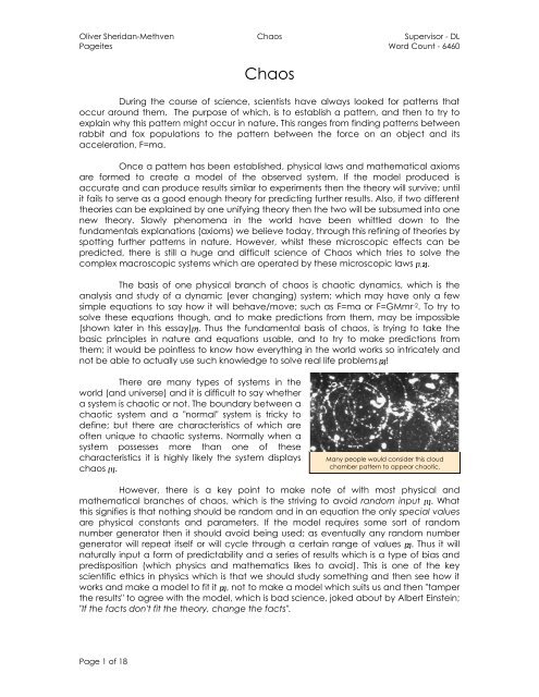
Many people would consider this cloud 

chamber pattern to appear chaotic. 

However, there is a key point to make note of with most physical and 

mathematical branches of chaos, which is the striving to avoid random input [1]. What 

this signifies is that nothing should be random and in an equation the only special values 

are physical constants and parameters. If the model requires some sort of random 

number generator then it should avoid being used; as eventually any random number 

generator will repeat itself or will cycle through a certain range of values [2]. Thus it will 

naturally input a form of predictability and a series of results which is a type of bias and 

predisposition (which physics and mathematics likes to avoid). This is one of the key 

scientific ethics in physics which is that we should study something and then see how it 

works and make a model to fit it [2], not to make a model which suits us and then "tamper 

the results" to agree with the model, which is bad science, joked about by Albert Einstein; 

"If the facts don't fit the theory, change the facts". 

Page 1 of 18



What we might consider to be a normal system to be like then, would be one 

where we could reasonably easily work out, either logically or mathematically, what 

state the system has been in, and will be in, after some period of time. Thus given the 

conditions at the start we could accurately predict what it will look like at a later point in 

time. However, this "forecasting" is only a small branch of physics, pointed out by Richard 

Feynman; "Physics like to think that all you have to do is say, these are the conditions, 

now what happens next". However, a chaotic system can be extremely difficult or even 

impossible to predict well [1,2,3], such as the three body problem (explained later). Thus a 

property of a chaotic system is the issue with predictability; if it is difficult to predict or 

approximate what a later state will look like, then the system may be chaotic. 

This property of unpredictability can be caused by either/all of these three 

qualities of the system: 

A. Sensitive dependence 

B. Feedback loops 

C. Unsolvable equations [1,3,7,8] 

The last of these, C, is the simplest one; if the equations which are used to 

describe how the system behaves cannot be solved to give an exact solution (e.g. most 

nonlinear differential equations) then it may be impossible to calculate what will happen. 

Most often though, to resolve this problem, approximations are made to make the 

equations simpler; so the equations might then merge together to provide a solution. 

Although the result it is not 100% correct it may be a good estimate. However, if this 

"guessing" needs to be repeated many times to extend the prediction further into the 

future, slowly the answer will become increasingly more unreliable [1,9]. 

The quality of sensitive dependence, A, is an issue not of the model's equations 

but rather of the data put into the model. Sensitive dependence arises with the 

uncertainty and error in a recorded value. If some data is input then a result is produced, 

however, as no data is 100% accurate [9], it is most likely a little bit off. Thus when a value 

is put in a range of values should be calculated, from the lowest possible value to the 

highest to give the spectrum of possible outcomes taking into account how wrong your 

measurements and data could be [9]. With many systems a little change in the data 

results in a little change in the result which is proportional to the error. This is the case of 

linear systems [3]. However, nonlinear systems are harder to work with because a little 

change in the data can result in a huge change in the outcome. Thus if there is a little 

error in the data there could be a huge variation in the results (technically quantified by 

Lyapunov exponents), thus if the data is not to a sufficient accuracy, the model could be 

unusable for making predictions [1]. James Gleick made the analogy to a pebble in a 

bowl and a pencil on a table. With the pebble in the bowl, if the pebble is in the bottom 

of the bowl then it will stay in the bottom, and if the data is wrong and the pebble is said 

to be an inch from the bottom then it will soon roll and settle into the bottom of the bowl 

and thus the system is not sensitive to it's initial conditions and it would be accurate for 

making predictions as to where the pebble will be. However, 

if you're trying to balance a pencil upright on its tip, then a 

tiny inaccuracy in the position of the top of the pencil can 

give many different results, and so this model will not be 

reliable for making predictions due to its sensitivity on data 

accuracy; which is an example of sensitive dependence [2]. 

This is one of the reasons why it is easy to stay balanced 

sitting a bath but difficult to walk on a tight rope! 

Page 2 of 18



The final feature of a feedback loop in a system, B, is often found hand in hand 

with sensitive dependence; commonly seen as two sides of the same coin. However, 

there are subtle differences between the two which are quite important. A feedback 

loop is often associated with an iterative solution to a problem, which might be forced by 

C. Thus if an error is present then it will still be present in the answer. The following state of 

the system is dictated by the previous state of the system when using iteration and so any 

uncertainty will be translated through the iterative feedback loop. Dependent on the 

system this can then be the cause of A but the fact that A is present doesn't imply that B 

is [1]. Thus B almost always forces A to occur, but A being present doesn't mean that B is 

(Figure1). 

Sensitive 

Dependence 

Figure1 

Normally Produces 

Sometimes Contains 

Feedback 

Loops 

The simplest system created which displays all of these characteristics was first 

discovered in biology and later analysed mathematically. This is the logistics map and 

was used initially to model a population of animals. What must happen is that the 

population must increase over time when it is small, so the first term was put in: 

F(X1) = λX0 

What this does is it increases the previous year's population, X0, by a fixed ratio, 

λ, to give the next years population, X1. However, this means that after enough time the 

population will become effectively infinite and bigger than it could possibly be. Thus a 

correctional term is introduced to bring down the population when it gets big and to 

boost it when it is small. NB the state of the population is between 0-1 for simplicity [1,2,3]. 

F(X1) = λX0(1-X0) Ξ λ(-X0 2 + X0) 

Thus if this feedback loop is iterated (Figure2) then it should hopefully settle into 

a stable population. NB as this population represents the state of the system, this 

forecasting function can be used in other systems in maths, physics etc. However, when 

this is done over a range of values for λ then whilst it appears there may be stability in low 

values, past a certain point it will split into repeating solutions. This means that the system 

is oscillating between two states in a regular cycle which is reasonable. However, this 

splitting (birefringence) can occur again and again as λ increase until suddenly there is 

no order in the answers and there is a chaotic system! How this chaos mathematically 

arises is symbolically shown by the iterative process beside the logistics map in Figure2 [7]. 

Page 3 of 18



X 唴 

_ 

F(X 1 ) = λ(-X 0 

2 + X 0 ) 

Figure2 

λ 

What the logistics map symbolises for chaotic dynamics is the fact that in some of 

even the most simple systems; which can have just two or three factors effecting it, 

where one of these factors is adjustable, then it can be adjusted to produce any of three 

system states. First of these states is the state where nothing is happening and any initial 

state will soon settle into a fixed state. The second is where the system will fall into an 

active steady state where it will either be doing a fixed motion or will be cycling through 

states regularly (demonstrated in a later experiment). The final implication of the logistics 

map is that if the correct parameter (λ) is chosen, then the system will be unpredictable 

and will fall into a system of chaos that will appear to have no pattern and therefore 

looks random [2,7]. 

When a system appears random the challenge is to then spot some sort of 

underlying pattern or trend; and to manipulate the data until such a pattern (and thus 

predictability) arises. Whilst many chaotic systems may not have an underlying pattern, a 

significant amount does. The task is to first find any strange attractors; which are points or 

trajectories through phase space. Phase space is just a graph of how the system is 

behaving as time goes by (Figure3) and where a certain point represents a 

characteristic, such as velocity or angle or potential energy etc. Thus one point could 

represent a system having a lot of kinetic energy when it is at such an angle whilst 

another point signifies another state the system can be in such as low kinetic energy but 

high temperature [1,2,3]. Thus if all paths through phase space always end up reaching a 

certain point then that point is a strange attractor. Similarly if a path continues orbiting a 

point in a circle for example, then the centre is a strange attractor. Finally, if all paths 

converge eventually into a certain path/trajectory (be it a straight line or a bizarrely 

shaped curve as in Figure3), even if initially off that path, then that trajectory is known as 

a strange attractor. 

Page 4 of 18



Figure3 

Strange Attractors 

Figure3 shows how the measurements of a system and how it is behaving over 

time (top row); e.g. velocity with time, translate into phase space diagrams (bottom row) 

of height with gradient. Here it is evident that where the top row may be unclear in 

displaying how the system is behaving and what it will do with time (most prominent in 

the top right plot), when transformed into a phase space diagram it can become 

apparent what the system is doing. Thus apparent randomness, in what appears to be a 

chaotic system, can be translated into predictability in phase space, allowing for a 

chaotic system to be made predictable [1,3]. 

The idea of there being underlying patterns in phase 

space which produce predictability, seems counterintuitive for 

chaotic systems. The fact that "randomness" can have patterns 

seems slightly illogical (and to an extent impossible) and thus 

an experiment was conducted to try to demonstrate this 

concept with real data collected from the lab, and not 

produced from theory. A very basic system encountered 

which was unexpectedly chaotic was that of the pendulum. 

For an equivalent James Gleick used the image of a child on a 

swing, which will be extended upon in the explanation of the 

experiment. 

If a child is on a swing and the swing is not moving 

then as time goes by the child will stay on the swing in the 

same position, which is obvious. If a child is then pushed once 

in the swing then they will oscillate to and from the same 

height, just at different angles on the swing (demonstrating the 

conservation of energy). Finally if friction is acknowledged then 

eventually the energy will dissipate from the system and the 

child will eventually come to a halt in the bottom of the swing 

position again. When these three processes are plotted in 

phase space (Figure4) it is much clearer to see the behaviour 

of the system and to spot the strange attractors in the system. 

NB even though the system is not yet chaotic, it has strange 

attractors in phase space [2]. 

In the frictionless system the swing will carry on 

swinging and the phase space will form a loop (Fiugre4) which 

Strange Attractors 

Figure4 

Page 5 of 18



demonstrates that after a certain period of time it will reach the same state. As it is then 

identical in state to how it was previously, it will follow the same course of action, and 

thus if a loop is formed it will continue in that loop forever. Equally, with the swing that has 

friction, it must eventually settle down to a fixed point which is when the swing has 

stopped [2] and so the phase space trajectory will always collapse into the origin 

(Fiugre13). 

However, a simple modification can be made to this system which quite 

unexpectedly introduces chaotic properties. This is to introduce a regular pushing force, 

such as a periodic torque on the swing. At first glance, this would seem just as regular as 

before, only just slightly more complicated mathematically. When a child is swinging, 

every time they reach the top of their return swing, they pull on the swing's rope (doing 

work on it and adding energy to the swing system) so that they stay in a regular swinging 

motion; where's the chaos in that? However, this is not a continuous and regular force; 

these are discrete and well timed packets of energy input specifically chosen for that 

frequency of swinging [2]. If the child were to do just the same rhythm of tugging on the 

rope on a longer swing, then they would pull at the wrong time, cause a jerk in the 

swing's motion, either speed up or slow down too quickly and would fall off. As will be 

shown later by the experiment, they may also swing through a full rotation and then 

suddenly stop at the bottom, which would certainly cause any child injury. 

Upon a technical analysis of what happens, is that although the pattern of 

forces applied may be in equilibrium, only some of the time, will this result in a system 

which is in equilibrium. This unexpected point was noted by James Gleick; "Even when a 

dampened, driven system is at equilibrium, it is not at equilibrium". This is due to the non 

linear relationship between the forces as time goes by [2,5]. The flow of energy in and 

energy out of the system has non linear equations, because the frictional torque is 

derived from the angular velocity, which changes with the angle of the swing as it goes 

from the bottom to the top of its arc. This is an example of how the system has a 

feedback loop and as we will see from the later experimental results, sensitive 

dependence. 

ΣT 

Φ 

L 

m 

Figure5 

m 

ω 

T 1 ,T 2 ,T 3 

The setup for the experiment was as follows 

(Figure5) [5]: 

For the experiment (in theory) there should be 

three sources of torque acting on the pendulum; T1, T2, T3 

[5]. The first is the torque from gravity which would 

produce simple harmonic motion (approximately for δΦ) 

provided it was the only force acting on the pendulum. 

The second is the torque due to friction which always 

works against the direction of the angular velocity. The 

final is the torque due to the driving force (child pulling 

on the swing's rope) adding torque in a periodic 

manner. 

Mathematically, these torques are given by: 

o T1 = -LmgSin(Φ)* 

o T2 = -kω † 

Commonly approximated to –LmgΦ to produce SHM 

Where k is a parameter value to determine the strength of 

the frictional torque 

Page 6 of 18



o T3 = ASin(λt) 

This provides an external periodic torque on the system 

NB *the negative values denote for the first torque that it always acts to bring 

the pendulum back to the rest position, against the orientation of Φ, and is inwards 

acting. † The second negative torque signifies that the friction always acts in the 

orientation opposing the angular velocity of the pendulum. 

Thus by the laws of rotational motion where: 

Iα = ΣT as I = mL 2 

mL 2 α = T1 + T2 + T3 

mL 2 α = -LmgSin(Φ) –kω + ASin(λt) [5] 

α = -gL -1 Sin(Φ) + (-kω + ASin(λt))m -1 L -2 [7] as ω = Φ' and α = Φ'' 

Φ'' = -gL -1 Sin(Φ) + (-kΦ' + ASin(λt))m -1 L -2 

The problem with these equations is that they cannot be solves explicitly to find 

the solution for Φ [7,8]. Thus there is no general solution for the angle with time, and 

therefore it is unpredictable with regards to a mathematically exact solution. This is due 

to the equation being a second and first order differential equation, which is nonlinear [8]. 

This can only be approximated, to guess a solution for a value of time, by performing an 

iterative approximation over δt periods. This will act to guess the position quite well, but as 

time goes by the guess will eventually become evermore unreliable. This demonstrates 

how this system is mathematically chaotic. In reality though, does it actually behave 

chaotically? The aim of the experiment was to discover if any strange attractors appear 

after analysis of the data; and whether this system of unsolvable equations produces 

reliability. The question is whether from the chaotic equations a regular system can be 

found? 

The experiment was aimed to resemble the computer simulation provided by 

source [5] as closely as possible (Figure6). There were initial problems with methods of 

recording the position of the end of the pendulum with the corresponding time by use of 

video tracking due to the speed of the pendulum. This was resolved with a device with a 

protruding axle which was attached to the pivot of the pendulum. The device has a 

relatively much lower rotational friction compared to the driving force device (motor) of 

the pendulum. Thus whilst this setup was not ideal, as the added friction was relatively 

minor effect, it could be neglected. The driving torque was provided by an electrical 

motor powered by a signal generator giving out an AC produced by a varying voltage 

which followed a sine wave. This produced a varying torque which exactly matched T3. 

NB this was verified by the cathode ray oscilloscope during the experiment. 

Page 7 of 18



Figure6 

The CRO (above) verified the voltage 

acting on the pendulum was a sine 

wave and that the signal generator 

(below) caused an AC through the 

motor. 

The motor here provided the driving 

torque to act on the pendulum. The 

nuts and bolts at the end 

approximate a pendulum as closely 

as possible. 

The blue device records the angle of 

the pendulum with time and has a 

very low frictional torque. The axes 

were joined together by the tube 

device at the top of the pendulum. 

NB – Whilst the essential principles for the pendulum were from [5], the experiment was designed entirely by myself. 

However, the experiment’s setup was constructed with the aid of the Charterhouse’s Physics technicians. Yet, all data was 

collected and analysed by myself. 

M 

CRO 

A 

C 

m 

Output data of angle v s 

time 

Φ vs t 

The pendulum was approximated as closely as it could by a light metal rigid 

rod. A mass of two large metal washers was bolted onto the end of the pendulum so that 

the bulk of the mass was at the end of the rod (approximating a pendulum). When the 

signal generator was switched on the data was then recorded into "data studio", and 

then moved to Microsoft Office Excel (Figure7). 

Figure7 

Page 8 of 18



The parameters of the experiment were: 

o The amplitude of the voltage from the signal generator and thus the 

maximum torque which could be driven into the pendulum. 

o The length and mass of the pendulum. 

o The frequency of the signal generator and thus how frequently the driving 

torque changes direction. 

Since the aim was to determine the nature of how birefringence from stable to 

chaotic might occur within the system due to the variation of just one of the parameters, 

two of the parameters were forces into set values. The only parameter which could be 

accurately changed through a relatively large range of values was the signal frequency, 

thus the others were kept at constant values during the collection of data. The signal 

amplitude was maintained at 5.6V + 0.1V and the length of the pendulum was always 

0.14m, which did not change during experiments, however, the error in this length was 

+0.003m. 

One of the preliminary experiments was to determine the nature of friction in 

the setup. Whether the frictional torque was a first, second, or even zero order 

polynomial function of the angular velocity. To discover this, a large blob of putty was 

formed into a ball around the axis, before all the data was collected, and was spun up 

to a very fast angular velocity (c200 rad/s), by a separate power supply. Then the power 

was disconnected and the observed angular deceleration was recorded (Figure8). 

Figure8 

Page 9 of 18



The significance of the straight line in Figure8 during the deceleration period 

shows that the frictional torque acting on the system acted on a zero order polynomial 

function of the angular velocity. What this meant was that there was an invariant 

(constant) frictional torque acting on the pendulum whenever it was in movement. 

Once this preliminary was conducted, the experimental data could be 

collected (Figure7). This was done over a set of values for the signal frequency from 

1.01Hz – 1.31Hz +0.01Hz. A typical spread sheet of data would contain a table of the 

initial conditions, the time, angle, angular velocity and a corrected angle. The corrected 

angle was a manipulation of the recorded angle; to transform it such that if the 

pendulum has rotated through 360 0 (2π c ) although the angles are recorded differently, 

then this new corrected angle would take the same value when the pendulum was in 

the same position. The reason for this should become clear after the analysis has been 

performed and the phase space trajectories plotted. 

Then a data set of the 

recorded angle against time was 

taken (Figure9) which could show 

how much the pendulum had 

rotated during the course of the 

data collection. What this shows is 

that during the blue run the 

pendulum had no preferred 

rotation, whilst in the purple run, 

the pendulum tended to 

repeatedly rotate through a full 

anticlockwise turn. This 

demonstrates how although all the 

conditions can appear the same to a 

high degree of accuracy, the results 

can soon diverge (Figure10), due to 

the sensitive feedback system which 

this proves to be. 

Figure9 

Figure10 

This sensitive dependence in 

the experiment shows how tiny 

discrepancies in the accuracy can 

result in differing outcomes and 

behaviours. This is best displayed with 

the corrected angles plot with time 

(Figure11). 

Demonstration of how identical states can quickly diverge 

into different final states. This was a weather simulation by 

Lorenz using only a few simple equations but the feedback 

loops caused this sensitive dependence. 

In Figure11 the top graph traces how the repeat run, the purple run, during the 

first five seconds almost identically follows the behaviour of the first run, the blue run. 

What this demonstrates is how the conditions in the start were (to a very high accuracy) 

the same. However, the middle graph follows how the two runs behaved in the 

proceeding five seconds, and how the two behaviours were starting to separate, shown 

by the waves becoming ever increasingly out of phase. Very soon after this difference 

had set in, it is clear to see how these two now slightly differing runs quickly become 

incoherent with respect to the other. During the fifteenth to the twentieth second 

(bottom graph), the two runs were in two completely different states, the blue run is 

following the motion of a normal pendulum, swinging back and forth, whilst the purple 

Page 10 of 18



run is swinging completely through a full rotation in a regular cycle. Thus although even 

the two runs had the same initial conditions, after a period of time (due to their sensitive 

dependence and feedback loops found in their equations) had settled into two different 

states/rhythms. 

0-5s 

5-10s 

Figure11 

15-20s 

There are ultimately three ways that the pendulum could behave (Figure12) 

depending on the frequency chose. If the frequency is too high then it will only cause a 

rapid and small vibration of the pendulum and overall this effect will cancel itself out, 

thus it will act approximately to a normal pendulum with friction and will come to a halt. 

This would cause an implicit trajectory through the phase space. This would also happen 

with a frequency that is too low, and then once the pendulum has settled into a 

stationary state the driving force would just tilt the pendulum slowly from side to side. 

Overall this would still produce an implicit trajectory. The second possibility, which is the 

most familiar to people, is to produce a symplectic trajectory. This would be where the 

frequency chosen would produce a regular oscillation, just as a child does on a swing to 

maintain reaching a constant height. In phase space this would form regular orbits and 

loops without touching the constraints (borders) of the phase space. The final possibility 

would be to produce an explicit 

trajectory where the pendulum would 

Figure12 

"randomly" gain speed and lose speed 

at certain points in the rotation. If a child 

were to do this on a swing then they 

would get higher and higher and 

possibly suddenly slow down at one 

point in the swing, then slow down to a 

stop again, giving a chaotic 

appearance when observed. Also they 

have the possibility of swinging over the 

top of the swing and then back round 

Explicit Implicit Symplectic 

Page 11 of 18



again and then returning to a normal pendulum action. In phase space this would be 

when the trajectory travels off the boundary in the phase space and then would return 

on the other side of the phase space. This is where the angle of the child changes from 

positive to negative once he crosses over the top of the swing. The purpose of correcting 

the angles was technically so that when a point went off of one boundary/edge, the 

corrected angle would cause the point to appear on the opposite side of the phase 

space. 

The transition from one of these trajectories into another type would be a form 

of birefringence of the system. Thus a further and more detailed aim was to see whether 

adjusting the frequency of the experiment's signal could produce these results. The first 

was to choose a very high frequency; which as explained earlier would have no overall 

effect but vibration. Thus the frequency was set to an excessively high frequency and 

was manually raised to a perpendicular position (90 0 ). Then it was released and the 

motion plotted and the 

trajectory through phase space 

traced (Figure13). 

What Figure13 displays 

is how the pendulum went from 

perpendicular and slowly swung 

through the centre four times, 

each time slowing down and 

then becoming stationary. 

Through phase space it traced 

the implicit trajectory, under the 

influence of the strange attractor 

at the origin. Therefore by 

adjusting the frequency the 

trajectory could be predicted. 

Thus at this frequency the 

chaotic system was easily 

approximated to a predictable 

one. Then the aim was then to 

construct the other two types of 

trajectories; symplectic and 

explicit, by causing a 

birefringence of the states 

through the variation of the 

signal frequency. 

Figure13 

The proceeding experiments were the runs where the frequency of the signal 

significantly affected the behaviour of the pendulum (i.e. not implicit trajectories); 

causing what appeared to be erratic behaviour. The first frequency (Figure14) was 

1.01Hz (there was a constant error in all frequencies of +0.01Hz) which initial caused an 

explicit trajectory (top left), behaving chaotically, until at around twenty seconds, it 

settled into an implicit trajectory (bottom left), following a regular pendulum motion. 

Overall the transition from chaotic into regular is best displayed by the angle time graph 

(top right) and gives the two overall trajectories (symplectic and explicit) through phase 

space (bottom right). 

Page 12 of 18



Explicit 

Symplectic 

Explicit 

Figure14 

Symplectic 

The significance of the pendulum having the capability of making the sudden 

transition from an explicit trajectory to a symplectic trajectory is that it is the 

manifestation of the feedback loop and the sensitive dependence. Where there was a 

feedback loop, the system was easily repeating the previous trajectory again and again. 

However, where it was a sensitive system, when the system diverged from this trajectory 

slightly, it was attracted by the strange attractor significantly enough to make the 

transition of trajectories into the symplectic trajectory. This demonstrates how tiny 

variations have the potential to cause large differences in states. 

Once this sensitivity within the system was established, the intension is to 

increase the frequency to find a birefringence of trajectories or a region of stability. At 

the frequencies around 1.14Hz (Figure15) the phase spaces began to have the majority 

of the trajectory following the explicit path and the minority having a symplectic form. 

Figure15 

Symplectic 

Explicit 

Page 13 of 18



Similar results were obtained with increasing frequencies until 1.31Hz was used 

(Figure16). When this frequency was applied an extremely regular explicit trajectory was 

formed. The pendulum swung very periodically through a full rotation in the same 

orientation. This was performed in a period four motion of the pendulum, due to the 

unique frequency that was able to resonate the pendulum, such that it produced a very 

regular oscillation pattern. 

Figure16 

The resulting phase space diagram in Figure16 represents how from the previous 

phase spaces, which appeared chaotic and without well defined trajectories (Fig14&15), 

a well selected frequency could produce a stable state. This is demonstrated by the 

extremely well defined trajectory which has great clarity (bottom graph in Figure16), 

forming a closed loop (joined at the edges of the phase space). However, how does this 

regularity arise from the chaotic birefringence 

and from amid the surrounding chaos? This can Figure17 

be said to be a unique solution/frequency 

which could be the one specially chosen to 

repeat this circuit of rotation; the 

correspondingly lower frequency is the one 

commonly used by a child on a swing [2]. 

However, from the logistics map which 

parallels this system, only the chaos arose. It 

didn't appear that there was any stability past 

the first onset of chaos. However, on further 

inspection there are streaks of stability 

(Figure17), emerging as clear lines amongst the 

black. These can correspond to frequencies 

which induce stability [1,2,3,7], such as 1.31Hz. 

These clear streaks represent the unique 

frequencies which can resonate the pendulum 

into a regular rhythm, such as 1.31Hz. 

Page 14 of 18



Figure18 

Computer Simulation by [5] 

Experimental Results 

So upon comparison of the 

experimental results to the computer 

simulation (Figure18) it is evident that the 

simulations can demonstrate many of the 

aspects of that occur in reality within the 

system. However, it would be difficult 

(almost impossible) to determine, from 

the four simple equations which govern 

the torque and the angular acceleration, 

the nature of the phase space 

trajectories and the strange attractors 

present. Secondly, it has proved to be a 

high quality manifestation of the logistics 

map and its qualities of birefringence and 

isolated regions of stability (1.31Hz) in such 

a relatively simply governed system 

(T1,T2,T3). 

Ultimately, this experiment 

demonstrates the capabilities that 

strange attractors have: that a plot in 

phase space can reduce the system's 

apparent randomness and 

unpredictability into order and patterns. From these patterns predictability can be 

induced which is the ultimate aim in experimental science; combining microscopic 

equations into macroscopic predictions, and the knowledge of what will happen next [2]. 

Throughout the history of physics and natural philosophy though, there has 

always been one topic that used to take precedence over all others. During the days 

when religion and science were intermingled, the stars and planets were of divine 

significance. The movement of the heavenly spheres (planets) and the study of 

astronomy were the professions of the educated few (natural philosophers, 

mathematicians and some members of the church). Beginning with the theory of a 

geocentric universe, this was changed by Nicolaus Copernicus, proposing the 

heliocentric model for calculations in his book, On the Revolution of Celestial Spheres. 

Following this Galileo Galilei more fully supported this idea until Johannes Kepler 

published in Harmony of the World the collected data which supported, to the point of 

proof, the heliocentric model. Finally the issue appeared to be settled definitively in Isaac 

Newton's Mathematical Principles of Natural Philosophy. This had proved to be the most 

problematic issue: predicting where the divine bodies will appear at a given time [4]. 

The key to Newton's success in resolving the issue definitively was to take 

Galileo's concept of inertia and extend upon it with mathematical description. These are 

known as Newton's three laws of motion which describe how things move. The first two 

laws can be described just by the second law; that when a force acts on a body its 

velocity will change. This is mathematically described by: 

F = dPdt -1 =ma 

The third law says for every impulse (F◦t) there is an equal and oppositely 

directed impulse. This law was not crucial though in his solution for a heliocentric model. 

Page 15 of 18



The ultimate key to the success of the Newtonian model was his first and second law and 

the knowledge of Kepler's laws of planetary motion. Newton used Kepler's third law to 

deduce his law of universal gravitation: 

F = -GMmr -2 the negative sign denotes the force is inwards acting [9]. 

From these laws there have been many derivations of how the planets move, 

which vary from the geometric proofs demonstrated in Principia and Feynman's Lost 

Lecture to algebraic proofs, using complicated calculus, such as in Mechanics and 

Vectors by Terry Heard [4,7,10]. The results from all of these are that the planets move in 

ellipses around the sun, the eccentricity of which can vary immensely; earth travels in a 

nearly circular orbit whilst Halley's Comet travels in a very eccentric orbit. Not only does 

theory predict this, but simulations support this (Figure19) and observations confirm this to 

a reasonable degree of accuracy. 

Figure19 

Here are two computer simulations using only the equations F = ma and F = -GMmr -2 which generate very accurate 

orbits (left) for earth and various comets (right). 

The key to the success in the predictions of these equations and simulations was 

the nature in which they were analysed. During all of these solutions there are only two 

bodies/planets, never more than two. The importance of this is that at all points in the 

orbit there is only once source of the gravitation force acting on any one body, which is 

the one produced by the other body. The significance is that during the geometrical 

analysis that all changes in velocity (acceleration) are in towards the other body directly. 

During the algebraic analysis, this means that the acceleration's component vector 

which is perpendicular to the axis connecting the two planets (a2) is equal to zero 

(Figure20). This is the fundamental principle 

from which all other derivations about the 

a 2 

planet's motion are made possible [4,7,10].The Figure20 

problem when three or more bodies of 

considerable mass are present is that the 

a 2 = 0 

principle that only centripetal acceleration 

exists (only a1) is frequently incorrect (i.e. a2 ≠ 

m 

0). Consequently then the geometric 

derivations and algebraic demonstrations 

a 1 

which relied on only a2 existing are reduced 

to false models [7]. 

M 

Page 16 of 18



The issue with a three or more body problem is that a new set of nonlinear 

equations are created, and a chaotic system is born (Figure20). Mathematically the 

equations are all unsolvable and can only be guessed by iterative functions (e.g. "the 

disturbing function"). However, normally with the huge masses, distances, velocities and 

forces involved, these models soon become unreliable. This unreliability is what induces 

the sensitive dependence within the system whilst the iterative process causes the 

feedback loops. This chaotic system is demonstrated by the simulation in Figure21, 

provided by source [6]. 

Figure21 

No Strange Attractors Exist 

The significance of three body problems having no strange attractors over the 

vast range of situations is that the ability of astronomy to produce reliable predictions 

becomes effectively impossible. When three bodies are present they could settle into 

some dynamic orbit within each other (which is irregular); they could collide with each 

other catastrophically! There is even the possibility that they call all collapse into each 

other and fling out one of the planets with a speed faster than the relative escape 

velocity. This makes efforts to forecast how our solar system formed and how it will 

continue, fundamentally ineffective. The exact course of our solar system, and even 

universe, can never be determined as a whole. No grand underlying pattern can 

possibly emerge and thus the accurate nature of the solar system, its future and past, is 

indeterminable [7]. 

Over the course of science, the purpose of investigation and experimentation 

has been to discover underlying patterns. From these trends, physical laws are produced 

in ever increasing accuracy. Our ability to forecast the most intricate events has grown in 

strength. However, whilst our knowledge of the microscopic world has grown, that of the 

macroscopic has reduced. With ever increasing knowledge of how systems behave on 

their own, it emerges that the giant mesh of systems that exist within the world form an 

ever decreasingly predictably structure. Chaos has proven that this is the case for even 

the most basic of systems such as the chaotic pendulum; extending through to 

historically the most philosophically important questions about the planets and their 

motions. This new and emerging science of chaos and chaotic dynamics has forced us 

to question the knowledge which we have traditionally believed to govern how things 

behave, finely summarised by James Gleick; "Knowledge of the fundamental equations 

no longer [seems] to be the right kind of knowledge at all". 

Page 17 of 18



Sources: 

[1] Chaos: A Very Short Introduction, Leonard Smith 

[2] Chaos, James Gleick 

[3] Introducing Chaos, Ziauddin Sardar & Iwona Abrams 

[4] Feynman's Lost Lecture, David & Judith Goodstein 

[5] http://myphysicslab.com/pendulum2.html - Chaotic Pendulum 

14/04/2010 

[6] http://myphysicslab.com/molecule3.html - Three Body Problem 

14/04/2010 

[7] Discussions with Ivan Hoffman DeVisme (IDV) 

[8] Discussions with Edward Reid (EJR) 

[9] Discussions with Dean Johnson (DRHJ) 

[10] Mechanics and Vectors, Terry Heard 

Page 18 of 18

Oliver Sheridan-Methven | PDF - Charterhouse

You also want an ePaper? Increase the reach of your titles

Delete template?

Save as template?