15-IJTPE-Issue14-Vol5-No1... - iotpe

International Journal on
“Technical and Physical Problems of Engineering”
(IJTPE)
Published by International Organization of IOTPE
ISSN 2077-3528
IJTPE Journal
www.iotpe.com
ijtpe@iotpe.com
March 2013 Issue 14 Volume 5 Number 1 Pages 103-107
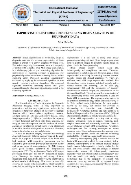
IMPROVING CLUSTERING RESULTS USING RE-EVALUATION OF
BOUNDARY DATA
M.A. Balafar
Department of Information Technology, Faculty of Electrical and Computer Engineering, University of Tabriz,
Tabriz, Iran, balafarila@tabrizu.ac.ir
Abstract- Image segmentation is preliminary stage in
diagnosis tools and the accurate segmentation of brain
images is crucial for a correct diagnosis by these tools.
Due to inhomogeneity, low contrast, noise and inequality
of content with semantic; brain MRI image segmentation
is a challenging job. A post processing algorithm for
improvement of clustering accuracy is proposed. The
proposed algorithm re-evaluates boundary data to reduce
clustering error. Proposed algorithm quantitatively
evaluated by applying the mentioned algorithm on two
recently reported clustering algorithms. The proposed
algorithm improved clustering results and gives
comparable results when user interaction is applied to the
clustering algorithms.
Keywords: Clustering, Brain, MRI.
I. INTRODUCTION
The identification of brain structures in Magnetic
Resonance Imaging (MRI) is very important in
neuroscience and has many applications, such as in the
detection of temporary changes in the brain’s electrical
function which causes seizure (epilepsy), tumours,
Multiple Sclerosis (MS) and Alzheimer’s disease. Brain
image segmentation [1, 2] is also crucial for the mapping
of brain functional activation onto brain anatomy, the
study of brain development, and the analysis of neuroanatomical
variability in normal brains [3]. In addition, it
is useful in the clinical diagnosis of psychiatric disorders,
treatment evaluation and surgical planning.
MRI is an important imaging technique for detecting
abnormal changes in different parts of brain at the early
stages. It is popular to obtain images of the brain with
high contrast. MRI acquisition parameters can be
adjusted to give different grey levels for different tissues
and various types of neuropathology [4]. MRI images
have good contrast compared to computerised
tomography (CT). The application of brain MRI imageprocessing
techniques has rapidly increased in recent
years. Nowadays, the capturing and storing of these
images are done digitally [5]. However, the interpretation
of their details is challenging. This matter is especially
observed in regions with abnormalities, which should be
identified by radiologists for future studies. Brain image
segmentation is a key task in many brain image
processing and diagnosis tools. Brain image segmentation
aims to partition images to different regions based on
given criteria for future processing.
Brain images usually contain noise [6],
inhomogeneity and complicated structures. Therefore,
segmentation is a challenging job. However, precise brain
segmentation is necessary for detecting tumours, oedema,
necrotic tissues and clinical diagnosis [7]. There are
different brain MRI image segmentation methods, like
thresholding, region growing, statistical models, active
control models and clustering. Due to noise [8],
inhomogeneity [9] and the complexity of intensity
distribution in medical images, the determination of the
threshold is difficult. Therefore, usually a combination of
the thresholding method with other methods is used for
brain MRI segmentation. The region-growing method is
an extension for thresholding, which adds connectivity to
it. This method needs initialisation for each region,
known as the seed, and inherits the problem of
thresholding to determine suite threshold for
homogeneity. Clustering methods are very common in
brain MRI segmentation. Fuzzy c-means (FCM) [10] and
statistical methods [11] are popular clustering methods.
Brain MRI segmentation is a key task in many
medical applications such as surgical planning, postsurgical
assessment and abnormality detection. Noise is
one of obstacles in brain MRI segmentation. Nowadays,
radiologists use fast scanning techniques to reduce
scanning times. These techniques raise the scanning noise
level in MRI systems. There are different de-noising
methods [12, 13] but they cannot totally remove noise
Intensity inhomogeneity [14] is another obstacle for
brain MRI segmentation which decrease similarity index.
Intensity inhomogeneity is the smooth intensity change
inside tissues. Inhomogeneity is hardly visible by the
user. But even invisible ones are enough to hamper
segmentation results. All inhomogeneity correction
methods obtain just estimation for an inhomogeneity bias
field and could not totally correct inhomogeneity.
Sometimes due to the inequality of content with
semantics, clustering methods fail to segment images
correctly. For these images, it is necessary to post-process
the clustering results.
103

International Journal on “Technical and Physical Problems of Engineering” (IJTPE), Iss. 14, Vol. 5, No. 1, Mar. 2013
II. BACKGROUND
A modified Gaussian Mixture GMM (EM1) [11] was
introduced by incorporating neighbourhood information
in the likelihood function and EM steps.
log( L( | X )) log p( x | ) log((1- ).
M
t t
j j i j
j1
Ki[ L]
rKi[1]
i1
. [ p ( x | ) * p])
1
t
p p j ( xr | j )
L
N
i
N
i1
where x r represents a neighbour of the pixel x i ,
K i [1],…,K i [L] denotes the set of neighbours of pixel x i
which is determined by a window centred on x i , L is the
number of neighbours, p is the average of distribution
t
values for neighbours of pixel x i , j denotes the
distribution parameters for the jth component at iteration
t
t, j denotes the mixture coefficient of component j at
iteration t, and parameter determines the weight of the
neighbourhood information and it is considered equal to
the variance of noise.
A modified EM, which is named as EM1, is proposed
to obtain the modified GMM parameters.
p( j | x , )
t1
j
Ki[ L]
t t
t
j[(1 ) p j ( xi | j ).* p j ( xr | j )]
L
t
rKi[1]
i j
M Ki[ L]
t t
t
j p j xi j p j xr j
j1 L
rKi[1]
t1
k
N
[(1 ) ( | ).* ( | )]
Ki[ L]
t
((1 ) x x ) p( j | x , )
i r i
i1 L
rKi[1]
N
t
p( j | xi
, )
i1
Ki[ L]
rKi[1]
N
i1
1
p( j | x , )
i1
t1 t1
T
i j xi j
.[(1 )( x )( )
{ p( j | x , ).
t1 t1
T
( xr j )( xr j
) ]}
L
i
t
N
Another improvement was introduced (EM2) [15].
The x i (average of neighbouring pixels around x i ) is
calculated prior to clustering.
log( L( | X )) log p( x | )
N
i1
N M
t t t
j j i j j i j
i1 j1
log( [(1 ) p ( x | ) p ( x | )])
p( j | x , )
i
t t t
t j j i j j j
i j M
t t t
j j i j j j
j1
[(1 ) p ( x | ) p ( x | )]
[(1 ) p ( x | ) p ( x | )]
i
t
(1)
(2)
(3)
(4)
(5)
(6)
N
t
((1 ) xi xi ) p( j | xi
, )
t1 i1
j
(7)
N
t
p( j | xi
, )
i1
N
t1
1
t
{ ( | , ).
k N p j xi
t i1
p( j | xi
, )
(8)
i1
t1 t1 T t1 t1
T
i j i j j j
.((1 )( x )( x ) ( x )( x ) )}
Sometimes, due to inhomogeneity, low contrast, noise
and inequality of content with semantics, automatic
methods fail to segment images correctly. Therefore, for
these images, it is necessary to use user-interaction to
correct a method’s error. However, robust semi-automatic
methods can be developed in which user-interaction is
minimized.
A user-interaction algorithm is introduced [15].
Sometimes, a clustered image either has pixels from two
or more tissues in one cluster or pixels from one tissue in
two or more clusters. To solve this problem, the user
selects clusters containing several tissues to be reclustered
into two sub-clusters. This process continues
until the user is satisfied. This means that the quality of
segmentation depends on the user. Then, to solve the
problem of several clusters for one tissue, the user selects
the clusters for each tissue.
III. METHODS
In this section, a new post-processing process which
re-evaluates boundary data to improve clustering results
is proposed. Proposed algorithm re-clusters each cluster
to reduce miss clustering rate.
A. Re-Evaluation of Boundary Data
User-interaction improves clustering performance but
makes clustering algorithms subjective and timeconsuming.
Also, algorithms lose their automatic nature
and it would be almost impossible to segment large
collections of image volumes using user-interaction. In
order to make algorithms automatic, but in the meantime
improve segmentation results, boundary data in clusters
are utilized. To improve clustering without userinteraction,
the boundary data in each cluster is reevaluated.
To do that, each cluster is re-clustered. Figure
1 demonstrates three clusters and their sub-clusters.
Figure 1. Three clusters and their sub-clusters,
underlined numbers are used for core parts
In Figure 1, sub-clusters with underlined numbers
represent the core parts of each cluster and other subclusters
are boundary parts. In order to specify the
situation of boundary data, core parts compete for
boundary parts. The steps of this algorithm are listed as
follows:
104

International Journal on “Technical and Physical Problems of Engineering” (IJTPE), Iss. 14, Vol. 5, No. 1, Mar. 2013
The input image is clustered to the n clusters, where n
is the number of target classes (here, the 4 clusters are
considered. Three represent the three tissues in the brain
while one is for the background). The output is the
clustered image.
Each cluster, except the background, is re-clustered.
In each cluster, the number of neighbouring clusters
specifies the number of boundary parts. Also, each cluster
will have one core part. Cluster number 2 is situated
between two clusters. Therefore, it is clustered into three
sub-clusters. However, clusters numbers 1 and 3 have just
one neighbouring cluster and are clustered into two subclusters.
Cluster number 1 is clustered into two subclusters,
numbers 11 and 12. Cluster number 2 is
clustered into three sub-clusters, numbers 21, 22 and 23.
Also, cluster number 3 is clustered into two sub-clusters,
numbers 31 and 32. The clusters and sub clusters are
ordered based on their mean intensity values.
In each cluster, the sub-clusters in the neighbourhood
of other clusters are considered as boundary parts while
the other sub-clusters are the core parts. The sub-clusters
11, 22 and 32 are considered as the core part and the
other sub-clusters are the boundary data for clusters
number 1, 2 and 3, respectively.
The core parts of the neighbourhood clusters compete
for their boundary parts. The core parts 11 and 22
compete for boundary parts 12 and 21. Steps 5 and 7 are
performed to specify the situation for boundary parts 12
and 21.
The abstract distances of centre of each boundary part
from the centres of the competing core parts are
calculated. The core part with less distance from a
boundary part is winner. The abstract difference between
the distances of a boundary part from two competing core
parts represents the winning degree for that boundary
part. For example, Figure 2 demonstrates the distances
between the core and boundary parts of clusters number 1
and 2. The abstract distances of boundary part 12 from
the centres of the competing core parts (11 and 22) are
denoted by d 1 and d 2 . The core part with less distance
from the boundary part centre is the winner. In
competition for boundary part 12, if d 1

International Journal on “Technical and Physical Problems of Engineering” (IJTPE), Iss. 14, Vol. 5, No. 1, Mar. 2013
Figure 5. The similarity index of EM1 with and without post-processing
when applied on 20 real images
Figure 3. Flowchart for the re-evaluation of boundary data
Figure 6. The similarity index of EM-2 with and without postprocessing
when applied on 20 real images
Figure 4. Two sub-process in follow chart for re-evaluation of boundary
data
V. CONCLUSIONS
In this paper, an automatic post processing algorithm
has been introduced. The performance of the proposed
algorithm on two recently reported clustering algorithm is
investigated. Sometimes due to the inequality of content
with semantics, clustering methods fail to segment
images correctly. For these images, it is necessary to
post-process the clustering results.
Figure 7. The average similarity index of the proposed algorithm when
applied on 20 real images
In last research a user-interaction algorithm for the
post-processing of clustering results are presented. The
algorithm uses user-interaction to improve clustering
results. In this paper, a new post processing algorithm is
proposed which improves clustering results by the reevaluation
of boundary data in each cluster. The
similarity index, r is used to evaluate algorithms.
Experiments demonstrate the effectiveness of the
proposed algorithm on improving clustering results in
terms of similarity index, r.
106

International Journal on “Technical and Physical Problems of Engineering” (IJTPE), Iss. 14, Vol. 5, No. 1, Mar. 2013
The focus of this research is on re-clustering on each
cluster. In future, we consider doing research for
changing the proposed post processing algorithm to
consider each boundary point and utilise optimizing
algorithms to improve clustering results.
REFERENCES
[1] M.A. Balafar, “Gaussian Mixture Model Based
Segmentation Methods for Brain MRI Images”, Artif.
Intell. Rev., pp. DOI 10.1007/s10462-012-9317-3, 2012.
[2] M.A. Balafar, “Fuzzy C-Mean Based Brain MRI
Segmentation Algorithms”, Artif. Intell. Rev., pp. DOI
10.1007/s10462-012-9318-2, 2012.
[3] X. Han, B. Fischl, “Atlas Renormalization for
Improved Brain MR Image Segmentation across Scanner
Platforms”, IEEE Transactions on Medical Imaging, Vol.
26, p. 479, 2007.
[4] D. Tian, L. Fan, “A Brain MR Images Segmentation
Method Based on SOM Neural Network”, 1st
International Conference on Bioinformatics and
Biomedical Engineering, pp. 686-689, 2007.
[5] P.L. Chang, W.G. Teng, “Exploiting the Self-
Organizing Map for Medical Image Segmentation”, 20th
IEEE International Symposium on Computer Based
Medical Systems, pp. 281-288, 2007.
[6] P. Coupe, J.V. Manjon, E. Gedamu, D. Arnold, M.
Robles, D.L. Collins, “Robust Rician Noise Estimation
for MR Images”, Medical Image Analysis, Vol. 14, pp.
483-493, 2010.
[7] L.O. Hall, A.M. Bensaid, L.P. Clarke, R.P.
Velthuizen, M.S. Silbiger, J.C. Bezdek, “A Comparison
of Neural Network and Fuzzy Clustering Techniques in
Segmenting Magnetic Resonance Images of the Brain”,
IEEE Transactions on Neural Networks, Vol. 3, pp. 672-
682, 1992.
[8] M.A. Balafar, “New Spatial Based MRI Image De-
Noising Algorithm”, Artifitial Intelligence Review,
DOI:10.1007/s10462-011-9268-0, pp. 1-11, 2011.
[9] M.A. Balafar, A.R. Ramli, S. Mashohor, “A New
Method for MR Grayscale Inhomogeneity Correction”,
Artificial Intelligence Review, Springer, Vol. 34, pp. 195-
204, 2010.
[10] S. Krinidis, V. Chatzis, “A Robust Fuzzy Local
Information C-Means Clustering Algorithm”, IEEE
Transactions on Image Processing, Vol. 19, pp. 1328-
1337, 2010.
[11] M.A. Balafar, A.R. Ramli, S. Mashohor, “Medical
Brain Magnetic Resonance Image Segmentation Using
Novel Improvement for Expectation Maximizing”,
Neurosciences, Vol. 16, pp. 242-247, 2011.
[12] C.S. Anand, J.S. Sahambi, “Wavelet Domain Non-
Linear Filtering for MRI Denoising”, Magnetic
Resonance Imaging, Vol. 28, pp. 842-861, 2010.
[13] M.A. Balafar, “Review of Noise Reducing
Algorithms for Brain MRI Images”, International Journal
on Technical and Physical Problems of Engineering
(IJTPE), Issue 13, Vol. 4, No. 4, pp. 54-59, December
2012.
[14] M.A. Balafar, “Review of Intensity Inhomogeneity
Correction Methods for Brain MRI Images”, Issue 13,
Vol. 4, No. 4, pp. 60-66, December 2012.
[15] M.A. Balafar, “Spatial Based Expectation
Maximizing (EM)”, Diagnostic Pathology, pp. 6-103,
2011.
BIOGRAPHY
Mohammad Ali Balafar was born in
Tabriz, Iran, in June 1975. He received
the Ph.D. degree in IT in 2010.
Currently, he is an Assistant Professor.
His research interests are in artificial
intelligence and image processing. He
has published 11 journal papers and 4
book chapters.
107