Abbreviated Interrupted Time-Series - Institute for Policy Research
Abbreviated Interrupted Time-Series - Institute for Policy Research
Abbreviated Interrupted Time-Series - Institute for Policy Research

Create successful ePaper yourself
Turn your PDF publications into a flip-book with our unique Google optimized e-Paper software.
<strong>Abbreviated</strong><br />
<strong>Interrupted</strong> <strong>Time</strong>‐<strong>Series</strong><br />
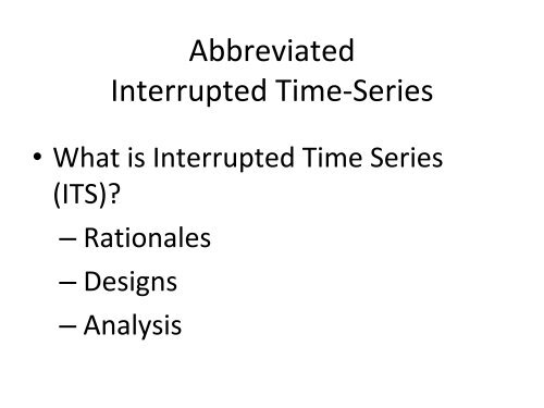
• What is <strong>Interrupted</strong> <strong>Time</strong> <strong>Series</strong><br />
(ITS)?<br />
– Rationales<br />
– Designs<br />
– Analysis
What is ITS?<br />
• A series of observations on the same dependent variable<br />
over time<br />
• <strong>Interrupted</strong> time series is a special type of time series<br />
where treatment/intervention occurred at a specific<br />
point and the series is broken up by the introduction of<br />
the intervention.<br />
• If the treatment has a causal impact, the postintervention<br />
series will have a different level or slope<br />
than the pre‐intervention series
The effect can be a change in<br />
intercept
The effects of charging <strong>for</strong> directory<br />
assistance in Cincinnati<br />
Number of Calls<br />
1000<br />
900<br />
800<br />
700<br />
600<br />
500<br />
400<br />
300<br />
200<br />
100<br />
0<br />
Intervention<br />
1962 1964 1966 1968 1970 1972 1974 1976<br />
Year
The effect can be a change in<br />
slope
Canada Sexual Assault Law Re<strong>for</strong>m<br />
3000<br />
2500<br />
Rape Re<strong>for</strong>m Law<br />
Number of Assaults<br />
2000<br />
1500<br />
1000<br />
500<br />
0<br />
1981 1982 1983 1984 1985 1986 1987 1988<br />
Year
The effect can be delayed in<br />
time.
The effects of an alcohol warning label on<br />
prenatal drinking<br />
0.8<br />
0.6<br />
Label<br />
Law<br />
Date<br />
0.4<br />
0.2<br />
0<br />
-0.2<br />
prenatal drinking<br />
-0.4<br />
Impact<br />
Begins<br />
-0.6<br />
Sep-86<br />
Jan-87<br />
May-87<br />
Sep-87<br />
Jan-88<br />
May-88<br />
Sep-88<br />
Jan-89<br />
May-89<br />
Sep-89<br />
Jan-90<br />
May-90<br />
Sep-90<br />
Jan-91<br />
May-91<br />
Sep-91<br />
Month of First Prenatal Visit
<strong>Interrupted</strong> <strong>Time</strong> <strong>Series</strong> Can Provide Strong Evidence<br />
<strong>for</strong> Causal Effects<br />
• Clear<br />
Intervention<br />
<strong>Time</strong> Point<br />
• Huge and<br />
Immediate<br />
Effect<br />
• Clear Pretest<br />
Functional<br />
Form + many<br />
Observations<br />
• No alternative<br />
Can Explain<br />
the Change
How well are these<br />
Conditions met in Most Ed <strong>Research</strong>?<br />
• The Box & Jenkins tradition require roughly 100<br />
observations to estimate cyclical patterns and error<br />
structure, but<br />
• This many data points is rare in education, and so we<br />
will have to deviate (but borrow from) the classical<br />
tradition.<br />
• Moreover,…
Meeting ITS Conditions in Educational<br />
<strong>Research</strong><br />
• Long span of data not available and so the pretest<br />
functional <strong>for</strong>m is often unclear<br />
• Implementing the intervention can span several<br />
years<br />
• Instantaneous effects are rare<br />
• Effect sizes are usually small<br />
• And so the need arises to develop methods <strong>for</strong><br />
abbreviated time series and to supplement them<br />
with additional design features such as a control<br />
series to help bolster the weak counterfactual<br />
associated with a short pretest time series
<strong>Abbreviated</strong> <strong>Interrupted</strong> <strong>Time</strong> <strong>Series</strong><br />
• We use abbreviated ITS loosely<br />
– series with only 6 to 50 time points<br />
• Pretest time points are important<br />
– valuable <strong>for</strong> estimating pre‐intervention growth<br />
(maturation)<br />
– control <strong>for</strong> selection differences if there is a<br />
comparison time series<br />
• Posttest <strong>for</strong> identifying nature of the<br />
response, especially its temporal persistence
• O X O<br />
Theoretical Rationales <strong>for</strong> more<br />
Pretest Data Points in SITS<br />
• Describes starting level/value ‐ yet fallibly so<br />
because of unreliability<br />
• But pre‐intervention individual growth is not<br />
assessed, and this is important in education
O O X O<br />
• Describes initial standing more reliably<br />
by averaging the two pretest values<br />
• Describes pre‐intervention growth<br />
better, but even so it is still only linear<br />
growth<br />
• Cannot describe stability of this<br />
individual linear growth estimate
O O O X O<br />
• Initial standing assessed even more reliably<br />
• Individual growth model can be better<br />
assessed—allow functional <strong>for</strong>m to be more<br />
complex, linear and quadratic<br />
• Can assessed stability of this individual<br />
growth model (i.e., variation around linear<br />
slope)
Generalizing to 00000000X0<br />
• Stable assessment of initial mean and slope<br />
and cyclical patterns<br />
• Estimation of reliability of mean and slope<br />
• Help determine a within‐person<br />
counterfactual<br />
• Check whether anything unusual is<br />
happening be<strong>for</strong>e intervention
Threats to Validity: History<br />
• With most simple ITS, the major threat to<br />
internal validity is history—that some other<br />
event occurred around the same time as the<br />
intervention and could have produced the<br />
same effect.<br />
• Possible solutions:<br />
– Add a control group time series<br />
– Add a nonequivalent dependent variable<br />
– The narrower the intervals measured (e.g.,<br />
monthly rather than yearly), the fewer the<br />
historical events that can explain the findings<br />
within that interval.
Threats to Validity: Instrumentation<br />
• Instrumentation: the way the outcome was<br />
measured changed at the same time that the<br />
intervention was introduced.<br />
– In Chicago, when Orlando Wilson took over the<br />
Chicago <strong>Policy</strong> Department, he changed the<br />
reporting requirements, making reporting more<br />
accurate. The result appeared to be an increase in<br />
crime when he took office.<br />
– It is important to explore the quality of the<br />
outcome measure over time, to ask about any<br />
changes that have been made to how<br />
measurement is operationalized.
Threat to SCV<br />
• When a treatment is implemented slowly and<br />
diffusely, as in the alcohol warning label study, the<br />
researcher has to specify a time point at which the<br />
intervention “took effect”<br />
– Is it the date the law took effect?<br />
– Is it a later date (and if so, did the researcher<br />
capitalize on chance in selecting that date)?<br />
– Is it possible to create a “diffusion model” instead<br />
of a single date of implementation?
Construct Validity<br />
• Reactivity threats (due to knowledge of being<br />
studied) are often less relevant if archival data<br />
are being used.<br />
• However, the limited availability of a variety<br />
of archival outcome measures means the<br />
researcher is often limited to studying just<br />
one or two outcomes that may not capture<br />
the real outcomes of interest very well
External Validity<br />
• The essence of external validity is exploring<br />
whether the effect holds over different units,<br />
settings, outcome measures, etc.<br />
• In ITS, this is only possible if the time series<br />
can be disaggregated by such moderators,<br />
which is often not the case.
Adding a Control Group <strong>Time</strong><br />
<strong>Series</strong>
O X O<br />
O O<br />
• Now we add a comparison group that did not<br />
receive treatment and we can<br />
• Assess how the two groups differ at one<br />
pretest<br />
• But only within limits of reliability of test<br />
• Have no idea how groups are changing over<br />
time
O O X O<br />
O O O<br />
• Now can test mean difference more stably<br />
• Now can test differences in linear growth/change<br />
• But do not know reliability of each unit’s change<br />
• Or of differences in growth patterns more<br />
complex than linear
O O O X O<br />
O O O O<br />
• Now mean differences more stable<br />
• Now can examine more than differences in linear<br />
growth<br />
• Now can assess variation in linear change <strong>for</strong><br />
each unit and <strong>for</strong> group<br />
• Now can see if final pre‐intervention point is an<br />
anomaly relative to earlier two
Example from Education: Project Hope<br />
• A merit‐based financial aid program in Georgia<br />
– Implemented in 1993<br />
– Cutoff of a 3.0 GPA in high school (RDD?)<br />
• Aimed to improve<br />
– Access to higher education<br />
– Educational outcomes<br />
• Control Groups<br />
– US data<br />
– Southeast data
Results:<br />
Percent of Students Obtaining High School GPA ≥ 3.00<br />
Percent of Students Reporting B or Better<br />
Percent<br />
90.00%<br />
88.00%<br />
86.00%<br />
84.00%<br />
82.00%<br />
80.00%<br />
78.00%<br />
76.00%<br />
74.00%<br />
Southeast<br />
US<br />
GA<br />
90<br />
92<br />
94<br />
96<br />
98<br />
2000<br />
Year
Results:<br />
Average SAT scores <strong>for</strong> students reporting high school GPA ≥<br />
3.00<br />
Avg SAT Scores, Students Reporting B or Better<br />
1,060<br />
1,040<br />
SAT Scores<br />
1,020<br />
1,000<br />
980<br />
960<br />
940<br />
Southeast<br />
US<br />
GA<br />
90<br />
92<br />
94<br />
96<br />
98<br />
2000<br />
Year
Adding a nonequivalent dependent<br />
variable to the time series<br />
NEDV: A dependent variable that is predicted not<br />
to change because of treatment, but is expected<br />
to respond to some or all of the contextually<br />
important internal validity threats in the same<br />
way as the target outcome
Example: British Breathalyzer Experiment<br />
• Intervention: A crackdown on drunk driving using a breathalyzer.<br />
• Presumed that much drunk driving occurred after drinking at pubs<br />
during the hours pubs were open.<br />
• Dependent Variable: Traffic casualties during the hours pubs were<br />
open.<br />
• Nonequivalent Dependent Variable: Traffic casualties during the<br />
hours pubs were closed.<br />
• Helps to reduce the plausibility of history threats that the decrease<br />
was due to such things as:<br />
– Weather changes<br />
– Safer cars<br />
– Police crackdown on speeding
Note that the outcome variable (open hours on weekend) did show an<br />
effect, but the nonequivalent dependent variable (hours when clubs<br />
were closed) did not show an effect.<br />
1600<br />
1400<br />
Traffic Casualties<br />
1200<br />
1000<br />
800<br />
600<br />
400<br />
200<br />
0<br />
1966<br />
1967<br />
Closed Hours<br />
Year<br />
1968<br />
Weekend
Example: Media Campaign to Reduce Alcohol Use<br />
During a Student Festival at a University (McKillip)<br />
• Dependent Variable: Awareness of alcohol abuse.<br />
• Nonequivalent Dependent Variables (McKillip calls<br />
them “control constructs”):<br />
– Awareness of good nutrition<br />
– Awareness of stress reduction<br />
• If the effect were due to secular trends (maturation)<br />
toward better health attitudes in general, then the<br />
NEDVs would also show the effect.
Only the targeted dependent variable, awareness of responsible<br />
alcohol use, responded to the treatment, suggesting the effect is<br />
unlikely to be due to secular trends in improved health awareness<br />
in general<br />
3.2<br />
3<br />
Good Nutrition<br />
Campaign<br />
Stress Reduction<br />
Responsible Alcohol Use<br />
Awareness<br />
2.8<br />
2.6<br />
2.4<br />
2.2<br />
2<br />
28-Mar 30-Mar 4-Apr 6-Apr 11-Apr 13-Apr 18-Apr 20-Apr 25-Apr 27-Apr<br />
Date of Observation
Adding more than one nonequivalent<br />
dependent variable to the design of SITS<br />
to increase internal validity
Example: Evaluating No Child Left Behind
NCLB<br />
• National program that applies to all public<br />
school students and so no equivalent group<br />
<strong>for</strong> comparison<br />
• We can use SITS to examine change in<br />
student test score be<strong>for</strong>e and after NCLB<br />
• Increase internal validity of causal effect by<br />
using 3 possible types of non‐equivalent<br />
groups or 3 types of contrasts <strong>for</strong> comparison
Contrast Type 1 & 2<br />
• Contrast 1: Test <strong>for</strong> NCLB effect nationally<br />
– Compare student achievement in public schools with<br />
private schools (both Catholic and non‐Catholic)<br />
• Contrast 2: Test <strong>for</strong> NCLB effects at the state level<br />
– Compare states varying in proficiency standards.<br />
• States with higher proficiency standards are likely<br />
to have more schools fail to make AYP and so more<br />
schools will need to “re<strong>for</strong>m” to boost student<br />
achievement
Contrast 1: Public vs Private Schools<br />
• Public schools got NCLB but private ones<br />
essentially did not<br />
–If NCLB is raising achievement in<br />
general, then public schools should do<br />
better than private ones after 2002<br />
• Hypothesis is that changes in mean,<br />
slope or both after 2002 will favor public<br />
schools
Hypothetical NCLB effects on public (red) versus<br />
private schools (blue)<br />
NAEP Test Score<br />
208<br />
200<br />
NCLB<br />
<strong>Time</strong>
Contrast 1: Public vs Private Schools<br />
• Two independent datasets: Main and Trend<br />
NAEP data can be used to test this<br />
• Main NAEP four posttest points. Data<br />
available <strong>for</strong> both Catholic and other<br />
private schools<br />
• Trend NAEP only one usable post‐2002<br />
point and then only <strong>for</strong> Catholic schools
Analytic Model<br />
• NCLB Public vs. Catholic school contrast<br />
• Model<br />
Y<br />
tj<br />
= β + β ( year)<br />
0<br />
+ β ( policy×<br />
group)<br />
6<br />
1<br />
• Low Power<br />
• Only 3 groups (public, Catholic, non‐Catholic private) with 8 time<br />
points. So only 24 degrees of freedom<br />
• Autocorrelation<br />
– Few solutions<br />
tj<br />
+ β ( group)<br />
2<br />
tj<br />
+ β ( policy)<br />
+ β ( policy×<br />
year×<br />
group)<br />
7<br />
+ β ( year×<br />
group)<br />
+ ε ,<br />
– Cannot use clustering algorithm because there are not enough groups<br />
– Robust s.e. used but results less conservative<br />
j<br />
3<br />
tj<br />
4<br />
tj<br />
tj<br />
tj<br />
+ β ( policy×<br />
year)<br />
5<br />
tj
Main NAEP <strong>Time</strong> <strong>Series</strong> Graphs<br />
Public vs. Catholic<br />
Public vs. Other Private
Main NAEP 4 th grade math scores by year:<br />
Public and Catholic schools
Main NAEP 4 th grade math scores by year:<br />
Public and Other Private schools
Difference in differences in Total change <strong>for</strong> 4 th Grade Math<br />
Analyses based on Main NAEP data<br />
Diff in Total ∆ (2009)<br />
4th Grade Math (All Data) 4th Grade Math (Exclude 1990)<br />
Coef. S.E. t Coef. S.E. t<br />
Public vs. Catholic 10.96 5.22 1.77+ 10.73 3.43 3.13*<br />
Public vs. Other Private 6.46 8.39 0.77 13.90 9.72 1.43<br />
+ p
Main NAEP 8 th grade math scores by year:<br />
Public and Catholic schools
Main NAEP 8 th grade math scores by year:<br />
Public and Other Private schools
Difference in differences in Total change <strong>for</strong> 8 th Grade Math<br />
Analyses based on Main NAEP data<br />
Diff in Total ∆ (2009)<br />
8th Grade Math (All Data) 8th Grade Math (Exclude 1990)<br />
Coef. S.E. t Coef. S.E. t<br />
Public vs. Catholic 2.91 6.64 0.44 0.26 5.57 0.05<br />
Public vs. Other Private 11.16 7.95 1.40 5.57 1.39 4.00*<br />
+ p
Trend NAEP <strong>Time</strong> <strong>Series</strong> Graphs<br />
Public vs. Catholic School Contrast<br />
(Other private school data unavailable and<br />
only 1 post‐intervention time point)
Trend NAEP 4 th grade math scores by year:<br />
Public and Catholic schools
Trend NAEP 8 th grade math scores by year:<br />
Public and Catholic schools
Difference in Differences in Mean Change in 2004 <strong>for</strong> Math<br />
Analyses based on Trend NAEP data<br />
Public vs. Catholic Contrast<br />
4th Grade Math<br />
8th Grade Math<br />
Coef. S.E. t Coef. S.E. t<br />
10.93 5.53 1.97* 7.26 2.03 3.58*<br />
* p
Public vs Private School Findings<br />
• All effects on 4 th and 8 th grade math are in<br />
right direction, and some statistically<br />
significant<br />
• No effect on 4 th grade reading but all are in<br />
the right direction (results not shown here)<br />
• This suggests that NCLB has a significant math<br />
effect nationally, but…
Concerns with Contrast 1<br />
• Possible low power due to low number of groups (3:<br />
public, Catholic, non‐Catholic private) with 8 time<br />
points<br />
– So only 24 degrees of freedom<br />
• Catholic sex abuse scandals in 2002 result in parents<br />
taking their children out of Catholic schools<br />
• No evidence that<br />
– school leavers caused a drop in average student<br />
achievement in Catholic schools or<br />
– public and other private school effects are due to<br />
transfers from Catholic schools<br />
• Data from other private schools provides a<br />
unconfounded replicate, but never stat sig.
Contrast 2: Comparing States that vary<br />
in Proficiency Standards<br />
• Some states set high standards <strong>for</strong> making AYP and<br />
so many schools fail and have to change their<br />
educational practices<br />
– (more serious NCLB implementers, higher dosage<br />
of treatment)<br />
• Other states set low standards and so do not have to<br />
change much<br />
– (less serious NCLB implementers, lower dosage of<br />
treatment)
Define Proficiency Standards Based on the<br />
Percentage of Students Deemed Proficient<br />
• To determine a state’s overall level of proficiency<br />
standard, we average the percentage of students<br />
deemed proficient across grades (4 th and 8 th grade)<br />
and across subjects (math and reading) using state<br />
assessment data from 2003<br />
• States that deemed less than 50% of students<br />
proficient have high proficiency standards<br />
• States that deemed 75% or more proficient are<br />
states have low proficiency standards<br />
• States between 50% and 75% are moderate
Evidence of Differing Standards<br />
High Proficiency Standard States<br />
Low Proficiency Standard States<br />
State State Test NAEP Test State State Test NAEP Test<br />
Arizona 46 24 Colorado 83 35<br />
Arkansas 46 25 Connecticut 76 39<br />
Cali<strong>for</strong>nia 36 22 Georgia 76 25<br />
District of Columbia 48 8 Minnesota 75 40<br />
Hawaii 31 21 Nebraska 80 33<br />
Kentucky 47 27 New Hampshire 76 39<br />
Maine 35 34 North Carolina 85 34<br />
Massachusetts 50 41 Tennessee 80 24<br />
Missouri 29 32 Texas 84 28<br />
Rhode Island 45 28 Virginia 75 35<br />
South Carolina 26 27 Wisconsin 77 35<br />
Washington 46 34<br />
Wyoming 39 35<br />
Mean 40 27 79 33<br />
1 Results are averaged across grades (4th and 8th grade), subjects (math and reading) in year 2003<br />
<strong>for</strong> state and NAEP assessment.<br />
Note: When state assessment data are missing in the grade examined, data from the next lower<br />
grade are used and if not available then data are from the next higher grade.<br />
Source: Consolidated State Per<strong>for</strong>mance Report and <strong>Institute</strong> of Education Science
So Contrast 2 is…<br />
• Compare states at three levels of standards ‐<br />
high, medium and low<br />
– Cut offs at 50% and 75% of students being<br />
proficient<br />
• Hypothesis is that in states with higher<br />
standards there should be more of a post‐<br />
2002 change in mean, slope or both<br />
• Using Main NAEP data from 1990 to 2009 <strong>for</strong><br />
Math and to 2007 <strong>for</strong> 4th grade Reading
Main NAEP <strong>Time</strong> <strong>Series</strong> Graphs<br />
States with High vs. Medium vs. Low<br />
Proficiency Standards
Adjusting <strong>for</strong> Autocorrelation<br />
• NCLB State Contrast<br />
• Option 1:<br />
– HLM model can control <strong>for</strong> autocorrelation<br />
Level 1:<br />
Y<br />
ti<br />
= γ + γ<br />
( year × policy)<br />
+ ε<br />
0i<br />
Level 2:<br />
γ<br />
0 i<br />
=<br />
β<br />
β<br />
00<br />
+ β<br />
1i<br />
( year)<br />
ti<br />
+ γ<br />
2i<br />
( policy)<br />
ti<br />
+ γ<br />
3i<br />
01<br />
( group<br />
( pupil _ teacher _ ratio ) + τ<br />
)<br />
i<br />
+ β<br />
03<br />
1 i<br />
= β10<br />
+ β11( group)<br />
i<br />
τ<br />
1i<br />
2<br />
= β<br />
20<br />
+ β<br />
21<br />
)<br />
i<br />
γ +<br />
γ<br />
i<br />
( group + τ<br />
2<br />
γ β β ( + τ<br />
3 i<br />
=<br />
30<br />
+<br />
31<br />
group)<br />
i 3i<br />
02<br />
( percent _ free _ lunch ) +<br />
i<br />
0i<br />
ti<br />
ti
],<br />
)<br />
(<br />
)<br />
(<br />
)<br />
(<br />
[<br />
)<br />
_<br />
_<br />
(<br />
)<br />
_<br />
_<br />
(<br />
)<br />
_<br />
(<br />
)<br />
_<br />
(<br />
)<br />
_<br />
(<br />
)<br />
_<br />
(<br />
)<br />
_<br />
(<br />
)<br />
_<br />
(<br />
)<br />
_<br />
(<br />
)<br />
_<br />
(<br />
)<br />
(<br />
)<br />
(<br />
)<br />
(<br />
3<br />
2<br />
1<br />
0<br />
13<br />
12<br />
11<br />
10<br />
9<br />
8<br />
7<br />
6<br />
5<br />
4<br />
3<br />
2<br />
1<br />
0<br />
ti<br />
ti<br />
i<br />
ti<br />
i<br />
ti<br />
i<br />
i<br />
i<br />
i<br />
ti<br />
ti<br />
ti<br />
ti<br />
ti<br />
ti<br />
i<br />
i<br />
ti<br />
ti<br />
ti<br />
ti<br />
year<br />
policy<br />
policy<br />
year<br />
ratio<br />
teacher<br />
pupil<br />
lunch<br />
free<br />
percent<br />
m<br />
group<br />
year<br />
policy<br />
h<br />
group<br />
year<br />
policy<br />
m<br />
group<br />
policy<br />
h<br />
group<br />
policy<br />
m<br />
group<br />
year<br />
h<br />
group<br />
year<br />
m<br />
group<br />
h<br />
group<br />
year<br />
policy<br />
policy<br />
year<br />
Y<br />
ε<br />
τ<br />
τ<br />
τ<br />
τ<br />
β<br />
β<br />
β<br />
β<br />
β<br />
β<br />
β<br />
β<br />
β<br />
β<br />
β<br />
β<br />
β<br />
β<br />
+<br />
×<br />
+<br />
+<br />
+<br />
+<br />
+<br />
+<br />
×<br />
×<br />
+<br />
×<br />
×<br />
+<br />
×<br />
+<br />
×<br />
+<br />
×<br />
+<br />
×<br />
+<br />
+<br />
+<br />
×<br />
+<br />
+<br />
+<br />
=<br />
• Full Model<br />
• Main Variables of Interest<br />
)<br />
_<br />
(<br />
8 h<br />
policy × group<br />
Analytic Model –Cont.<br />
β<br />
ti<br />
h<br />
group<br />
year<br />
policy )<br />
_<br />
(<br />
10 ×<br />
×<br />
β
Adjusting <strong>for</strong> Autocorrelation<br />
• Option 2:<br />
• Fixed effects model because we are looking at<br />
the entire population of states<br />
– Use cluster option in stata<br />
Y<br />
ti<br />
= β + β ( policy)<br />
0<br />
+ β ( policy × group _ h)<br />
5<br />
+ β ( policy × year × group _ h)<br />
7<br />
+ β ( percent _<br />
9<br />
1<br />
ti<br />
+ β ( policy×<br />
year)<br />
2<br />
ti<br />
free _ lunch)<br />
+ β ( policy × group _ m)<br />
ti<br />
6<br />
ti<br />
+ β<br />
+ β ( year × group _ h)<br />
+ β ( policy×<br />
year × group _ m)<br />
10<br />
8<br />
ti<br />
3<br />
( pupil _ teacher _ ratio)<br />
ti<br />
ti<br />
ti<br />
+ β ( year × group _ m)<br />
ti<br />
i<br />
4<br />
+ μ + τ + ε<br />
t<br />
ti<br />
,<br />
ti
Main NAEP 4 th grade math scores<br />
by year and proficiency standards
Main NAEP 8 th grade math scores<br />
by year and proficiency standards
Difference in differences in 2009 Total change <strong>for</strong> Math<br />
Analyses based on Main NAEP data<br />
4th Grade Math<br />
8th Grade Math<br />
Coef. S.E. t Coef. S.E. t<br />
High vs. Low Proficiency Standards<br />
Diff in Total ∆ (2009) 7.38 3.33 2.22* 6.97 3.38 2.06*<br />
+p
Contrast 2 Study Conclusions<br />
• NCLB increased<br />
– 4 th Grade Math<br />
– 8 points.<br />
– 6 months of learning<br />
– .26 SD<br />
– .21 Pct<br />
– 8 th grade math<br />
– 8 points<br />
– 12 months of learning<br />
– .19 SD<br />
– .20 pct<br />
– 4 th Grade Reading<br />
• No significant effect <strong>for</strong> either contrast but all are<br />
in the hypothesized direction
Overall Conclusions<br />
• Similar results obtain from both strategies:<br />
– significant 4 th and 8 th grade math effects but not <strong>for</strong><br />
reading<br />
• Viable internal threats are factors independent of NCLB<br />
that changed in 2002 and are correlated with both the<br />
public/private and the high/low proficiency contrasts<br />
• Most alternative interpretations do not apply to both<br />
strategies, and this should reduce concerns about<br />
internal validity<br />
• A few are shared (e.g., changes in math standards in<br />
public schools in 2002). These are discussed in the paper<br />
and shown to highly unlikely.
Contrast 3:<br />
Dee & Jacob
Basic Insight of D & J<br />
• NCLB passed in 2002 and is a system of accountability by<br />
per<strong>for</strong>mance standards with inevitable sanctions <strong>for</strong><br />
school failure<br />
• Some states had such a system earlier ‐ e.g, via<br />
Improving American Schools Act<br />
• States whose accountability system pre 2002 had no<br />
sanctions then become “treatment” group that gets<br />
consequential accountability (CA) via NCLB in 2002<br />
• States with systems that had sanctions pre‐2002 then<br />
become a comparison group post 2002
Basic Method of D & J<br />
• Prior studies can be used to determine which<br />
states did and did not have accountability system<br />
pre 2002<br />
• Dee & Jacob uses Hanushek’s measure<br />
• Main NAEP provides the pre‐intervention (2002)<br />
and post‐intervention time‐series <strong>for</strong> both<br />
reading and math<br />
• Hypothesis again is that NCLB should increase<br />
mean or slope or both after 2002 by more in<br />
states without a prior accountability system
D & J Results: 4 th Grade Math
D & J Results: 8 th Grade Math
Dee and Jacob Results<br />
• Similar causal findings to Wong,<br />
Cook & Steiner<br />
• Strong Evidence of a 4 th Grade Math<br />
Effect<br />
• Some evidence of 8 th Grade Math<br />
Effect<br />
• No Reading Effect
Two Causal Mechanisms<br />
• D & J claim results due to NCLB requiring some states to insert<br />
sanctions into their accountability systems in 2002 ‐ the<br />
consequential accountability mechanism (CA)<br />
• WC&S claim their results due to higher proficiency standards<br />
after 2002 imposing more sanctions and school change<br />
compared to states with lower proficiency standards ‐ the<br />
proficiency standards mechanism (S)<br />
• Correlation between two ‐ our measure and Hanushek’s ‐ is<br />
.05. So independent mechanisms.<br />
• How do the two combined relate to reading?
4 th Grade Reading
Differences in differences in total change post‐NCLB<br />
4 th Grade Reading<br />
Coef. S.E. t<br />
Wong et. al. vs. Dee and Jacob<br />
Diff in Total ∆ by 2009 (S+CA) 5.60 2.50 2.24 *<br />
Diff in Total ∆ by 2009 (S) 1.34 2.67 0.50<br />
Diff in Total ∆ by 2009 (CA) 1.98 2.56 0.78<br />
Wong (median) vs. Dee and Jacob (all)<br />
Diff in Total ∆ by 2009 (S+CA) 4.19 1.68 2.49 *<br />
Diff in Total ∆ by 2009 (S) 1.96 1.80 1.09<br />
Diff in Total ∆ by 2009 (CA) 2.05 1.66 1.24<br />
Interaction Effect 0.18 2.18 0.08<br />
+p
The Use of Multiple Comparison Groups<br />
and Replications<br />
• ALL three ITS contrasts point to a clear math effect<br />
– public vs. private<br />
– high vs. low standards<br />
– early versus late CA<br />
• When Standards and CA are combined, a modest reading<br />
effect appears in states that have a new sanction system and<br />
set high standards compared to states that already have a<br />
sanction system in place but set low standards after 2002.
Why did we need multiple<br />
comparison TS?
Adding Treatment Introduction<br />
and Removal: Examples from<br />
<strong>Research</strong> on Students with<br />
Disabilities
Example: Ayllon et al., A Behavioral Alternative<br />
to Drugs <strong>for</strong> Hyperactive Students<br />
• Drugs control hyperactivity, but can interfere<br />
with academic per<strong>for</strong>mance<br />
• Ayllon et al. used a behavioral intervention to<br />
try to control hyperactivity while improving<br />
academic per<strong>for</strong>mance as measured by<br />
– Math<br />
– Reading
Medication<br />
decreased<br />
hyperactivity, but<br />
also affected<br />
academic<br />
per<strong>for</strong>mance.<br />
Removal of<br />
medication<br />
increased<br />
hyperactivity<br />
but allowed<br />
academic<br />
per<strong>for</strong>mance to<br />
recover a bit.<br />
The behavioral<br />
rein<strong>for</strong>cement<br />
program reduced<br />
hyperactivity but<br />
allowed academic<br />
per<strong>for</strong>mance to<br />
increase even more.
Multiple Baselines on Different<br />
Dependent Variables
Example: Chorpita<br />
• A child with difficulties attending school, with<br />
symptoms including<br />
– Somatic complaints<br />
– Tantrums and anger<br />
– Crying<br />
• Intervention was a behavioral extinction and<br />
rein<strong>for</strong>cement schedule<br />
• Multiple baseline adding treatment <strong>for</strong> each of<br />
the three symptoms over time.
Initially, only somatic<br />
complaints were targeted.<br />
Then, both somatic<br />
complaints and<br />
anger/tantrums were<br />
targeted.<br />
Finally, all three sets of<br />
symptoms were targeted<br />
in the third phase.
Multiple Baselines on Different Units
Example: Bland<strong>for</strong>d and Lloyd<br />
• Two learning disabled boys<br />
• Intervention: A self‐instructional card with seven<br />
instructions on how to improve handwriting.<br />
• Outcome: Percent of possible points on a<br />
handwriting test<br />
• Multiple Baseline: Intervention was introduced at<br />
two different times <strong>for</strong> the two boys.
The effects of screening <strong>for</strong><br />
phenylketonuria retardation<br />
PKU Retardation<br />
Admissions<br />
7<br />
6<br />
5<br />
4<br />
3<br />
2<br />
1<br />
0<br />
PKU Retardation<br />
Admissions<br />
3.5<br />
3<br />
2.5<br />
2<br />
1.5<br />
1<br />
0.5<br />
0<br />
47-<br />
49<br />
50-<br />
52<br />
53-<br />
55<br />
56-<br />
58<br />
59 60 61 62 63 64 65 66 67 68 69 70 71<br />
47-<br />
49<br />
50-<br />
52<br />
53-<br />
55<br />
56-<br />
58<br />
59 60 61 62 63 64 65 66 67 68 69 70 71<br />
PKU Screening Adopted in 1962<br />
PKU Screening Adopted in 1963<br />
PKU Retardation<br />
Admissions<br />
6<br />
5<br />
4<br />
3<br />
2<br />
1<br />
0<br />
47-<br />
49<br />
50-<br />
52<br />
53-<br />
55<br />
56-<br />
58<br />
59 60 61 62 63 64 65 66 67 68 69 70 71<br />
PKU Screening Adopted in 1964<br />
PKU Retardation<br />
Admissions<br />
7<br />
6<br />
5<br />
4<br />
3<br />
2<br />
1<br />
0<br />
47-<br />
49<br />
50-<br />
52<br />
53-<br />
55<br />
56-<br />
58<br />
59 60 61 62 63 64 65 66 67 68 69 70 71<br />
PKU Screening Adopted in 1965
Analyses <strong>for</strong> Short <strong>Time</strong> <strong>Series</strong><br />
• Early proposals to use ordinary least squares<br />
statistics<br />
• The above ignores the fact that times series<br />
data are auto‐correlated
Multilevel Models: Current Work<br />
• Applying multilevel models to these data allows <strong>for</strong><br />
different behavior patterns across cases, and can<br />
account <strong>for</strong> those differences using characteristics of<br />
the cases in the model.<br />
• We began analyses with a 1‐phase study (treatment<br />
only), then 2‐phase studies (AB), and are now<br />
working to model 4‐phase studies (ABAB).<br />
• At each stage, we’ve discovered new technical issues<br />
to be considered and accommodated.<br />
90
Potential advantages of using HLM to analyze and<br />
synthesize SCD data both within and across studies:<br />
1. Appropriately considers observations as nested within<br />
cases<br />
2. Does not require that all cases have the same number of<br />
observations or the same spacing of observations over<br />
time<br />
3. Allows treatment effects to vary across cases, attempting<br />
to explain any heterogeneity of effects by adding subject<br />
or setting characteristics to the model<br />
4. Can provide reliable estimates even with only few data<br />
points per cases<br />
91
Potential drawbacks of using HLM to analyze<br />
and synthesize SCD data (both within and<br />
across studies):<br />
1. Can be intimidating to some researchers<br />
2. Can be difficult to estimate parameters when models<br />
get complex<br />
• Especially when number of time points and<br />
number of cases is small.<br />
• Especially when modeling quadratic terms.<br />
• Especially when using a fully random effects<br />
model.<br />
92
Example: Stuart 1967<br />
• 8 time series, one on each of 8 people<br />
• Weight loss intervention over one year<br />
• Wt loss in pounds as dv<br />
• Here are the 8 time series:
Stuart Data<br />
Example (Stuart, 1967)<br />
94
Level 1 (time within persons)<br />
95
Level 2 data: Persons<br />
Level-2 data (subject characteristics):<br />
96
An Example of Modeling These Data in<br />
HLM<br />
Building a Simple Linear Model in HLM:<br />
POUNDS ij = π 0 + π 1 *(MONTHS12) +e ij<br />
π 0 = average ending weight<br />
π 1 = average rate of change in weight per month<br />
97
HLM: Linear Model Estimates<br />
Final estimation of fixed effects:<br />
Standard Approx.<br />
Fixed Effect Coefficient Error T-ratio d.f. P-<br />
value<br />
----------------------------------------------------------<br />
For INTRCPT1,P0<br />
INTRCPT2, B00 156.439560 5.053645 30.956 7 0.000<br />
For MONTHS12 slope, P1<br />
INTRCPT2, B10 -3.078984 0.233772 13.171 7 0.000<br />
----------------------------------------------------------<br />
The outcome variable is POUNDS<br />
----------------------------------------------------------<br />
POUNDS ij ≈ 156.4 – 3.1*(MONTHS12) +e ij<br />
98
Quadratic Model Building<br />
POUNDS ij = π 0 + π 1 *(MONTHS12)+ π 2 *(MON12SQ)+e ij<br />
π 0 = average ending weight<br />
π 1 = average rate of change in weight per month near the end of<br />
the study<br />
π 2 = average rate of change in slope, or effect of time on weight<br />
loss<br />
99
HLM Output from Quadratic Model:<br />
Final estimation of fixed effects:<br />
Standard Approx.<br />
Fixed Effect Coefficient Error T-ratio d.f. P-value<br />
-----------------------------------------------------------<br />
For INTRCPT1, P0<br />
INTRCPT2, B00 158.833791 5.321806 29.846 7 0.000<br />
For MONTHS12 slope, P1<br />
INTRCPT2, B10 -1.773039 0.358651 -4.944 7 0.001<br />
For MON12SQ slope, P2<br />
INTRCPT2, B20 0.108829 0.021467 5.070 7 0.001<br />
-----------------------------------------------------------<br />
The outcome variable is POUNDS<br />
-----------------------------------------------------------<br />
POUNDS ij ≈ 158.8 – 1.8(MONTHS12) + 0.1*(MON12SQ) + e ij<br />
10
Comparing Models<br />
Stuart (1967) – Actual Data<br />
Linear Model Prediction (HLM)<br />
215.7<br />
226.2<br />
196.2<br />
203.3<br />
POUNDS<br />
180.5<br />
POUNDS<br />
176.7<br />
157.2<br />
157.7<br />
134.8<br />
-12.60 -9.30 -6.00 -2.70 0.60<br />
MONTHS12<br />
137.8<br />
-12.00 -9.00 -6.00 -3.00 0<br />
MONTHS12<br />
Quadratic Model Prediction (HLM)<br />
219.2<br />
199.1<br />
• Even graphically, the quadratic<br />
model looks to be a better fit to the<br />
original data.<br />
POUNDS<br />
179.0<br />
158.8<br />
138.7<br />
-12.00 -9.00 -6.00 -3.00 0<br />
MONTHS12<br />
• Patients lost weight at a faster rate<br />
at the beginning of treatment and<br />
at a slower rate towards the end of<br />
the one-year treatment.
So Simple: What Could Go Wrong?<br />
• HLM has problems<br />
• when all effects are random<br />
• with autoregressive model<br />
• WinBUGS works well, but harder to learn<br />
• Fortunately, the WinBUGS estimates closely<br />
approximate the HLM estimates.<br />
10
What Else Could Go Wrong?<br />
• Different studies have time series that use<br />
different outcome metrics (both between and<br />
often within studies)<br />
– Counts, rates, means, ratings, totals, etc.<br />
– With timed or untimed administration<br />
– With constant or variable number of “items”
Problematically<br />
• Different combinations of these have different<br />
distributions, e.g.,<br />
– Binomial <strong>for</strong> counts with fixed n of trials<br />
– Poisson <strong>for</strong> rates with variable n of trials<br />
• HLM usually assumes normally distributed data.<br />
– One can change this, but<br />
– It isn’t clear HLM how can allow different distributions <strong>for</strong><br />
different studies in the same meta‐analysis.
So We Are Working On<br />
• Categorizing the different kinds of metrics and<br />
associated distributions, and<br />
• Seeing whether they can be modeled correctly<br />
in programs like HLM or WINBUGS.
Do you have any examples to share with us?
Summary<br />
• ITS is a very powerful design, but feasibility depends<br />
on the availability of a good archived outcome, or<br />
ability to gather original data<br />
• Much prior in<strong>for</strong>mation is available in education, at<br />
individual, cohort and school levels<br />
• But it is not much used in education outside of<br />
special education with individual cases. Why?<br />
Its use is not recommended without a comparison<br />
time series due to unclear extrapolations from<br />
pretest alone and uncertainty about when an effect<br />
should appear