Simplified Nyquist Criterion

5.6 Stability test and controller setting with the frequency response of the
open control loop 153
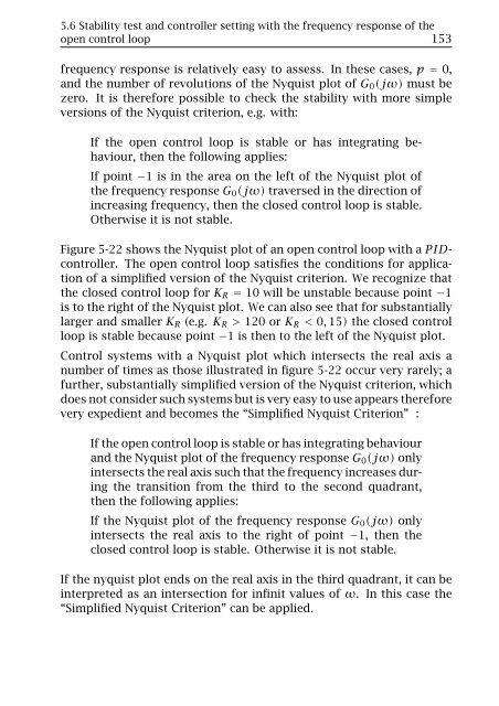
frequency response is relatively easy to assess. In these cases, p = 0,
and the number of revolutions of the Nyquist plot of G 0 (jω) must be
zero. It is therefore possible to check the stability with more simple
versions of the Nyquist criterion, e.g. with:
If the open control loop is stable or has integrating behaviour,
then the following applies:
If point −1 is in the area on the left of the Nyquist plot of
the frequency response G 0 (jω) traversed in the direction of
increasing frequency, then the closed control loop is stable.
Otherwise it is not stable.
Figure 5-22 shows the Nyquist plot of an open control loop with a PIDcontroller.
The open control loop satisfies the conditions for application
of a simplified version of the Nyquist criterion. We recognize that
the closed control loop for K R = 10 will be unstable because point −1
is to the right of the Nyquist plot. We can also see that for substantially
larger and smaller K R (e.g. K R > 120 or K R < 0, 15) the closed control
loop is stable because point −1 is then to the left of the Nyquist plot.
Control systems with a Nyquist plot which intersects the real axis a
number of times as those illustrated in figure 5-22 occur very rarely; a
further, substantially simplified version of the Nyquist criterion, which
does not consider such systems but is very easy to use appears therefore
very expedient and becomes the “Simplified Nyquist Criterion” :
If the open control loop is stable or has integrating behaviour
and the Nyquist plot of the frequency response G 0 (jω) only
intersects the real axis such that the frequency increases during
the transition from the third to the second quadrant,
then the following applies:
If the Nyquist plot of the frequency response G 0 (jω) only
intersects the real axis to the right of point −1, then the
closed control loop is stable. Otherwise it is not stable.
If the nyquist plot ends on the real axis in the third quadrant, it can be
interpreted as an intersection for infinit values of ω. In this case the
“Simplified Nyquist Criterion” can be applied.

160 Controller setting and stability of control loops
5.6.3 Controller design in the Bode diagram
For the practical treatment of linear control systems the representation
of frequency responses in the Bode diagram is preferred above that by
the Nyquist plots because the former method is simpler by far. The
statements on the stability of a closed loop provided by the Nyquist
criterion can be transferred to the representation of the frequency response
of the open control loop in the Bode diagram. This shall only
be dealt with in the following text within the context of the “Simplified
Nyquist Criterion”.
As illustrated in figure 5-26, we can, for stability testing with the “Simplified
Nyquist Criterion” determine the frequency ω π from the phase
response with the definition ϕ 0 (ω π ) =−π and check whether the amplitude
of the frequency response |G 0 (jω π )| is less than one. Alternatively,
with the definition |G 0 (jω d )|=1 we can obtain from the amplitude
response the frequency ω d and check whether the phase angle
ϕ 0 (ω d ) is greater than −π.
We must ensure in every case that the “Simplified Nyquist Criterion” is
applicable.
Summarizing, the “Simplified Nyquist Criterion” for the application in
the Bode diagram gives:
If the open control loop is stable or has integrating behaviour
and the phase response of its frequency response in the Bode
diagram intersects the lines −180 ◦ − n · 360 ◦ with a negative
slope only, then the following applies:
If the amplitude of the frequency response |G 0 (jω π )| is less
than one at frequency values for which the phase response
gives ϕ 0 (ω π ) =−180 ◦ − n · 360 ◦ , then the closed control
loop is stable. Otherwise it is not stable.
For the “Simplified Nyquist Criterion” the point where the phase response
is just tangent to the line −180 ◦ − n · 360 ◦ for infinit values of
ω has to be considered.
Figure 5-26 also shows that it is possible to obtain the gain margin
from the amplitude response |G 0 (jω π )| and the phase margin from
the phase response ϕ 0 (ω d ).