Expansions for statistics involving the mean absolute deviations

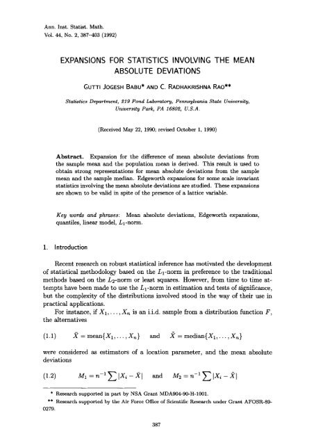
Ann. Inst. Statist. Math. 

Vol. 44, No. 2, 387-403 (1992) 

EXPANSIONS FOR STATISTICS INVOLVING THE MEAN 

ABSOLUTE DEVIATIONS 

GUTTI JOGESH BABU* AND C. RADHAKRISHNA RAO** 

Statistics Department, 219 Pond Laboratory, Pennsylvania State University, 

University Park, PA 16802, U.S.A. 

(Received May 22, 1990; revised October 1, 1990) 

Abstract. Expansion for the difference of mean absolute deviations from 

the sample mean and the population mean is derived. This result is used to 

obtain strong representations for mean absolute deviations from the sample 

mean and the sample median. Edgeworth expansions for some scale invariant 

statistics involving the mean absolute deviations are studied. These expansions 

are shown to be valid in spite of the presence of a lattice variable. 

Key words and phrases: Mean absolute deviations, Edgeworth expansions, 

quantiles, linear model, Ll-norm. 

1. Introduction 

Recent research on robust statistical inference has motivated the development 

of statistical methodology based on the Ll-norm in preference to the traditional 

methods based on the L2-norm or least squares. However, from time to time attempts 

have been made to use the Ll-norm in estimation and tests of significance, 

but the complexity of the distributions involved stood in the way of their use in 

practical applications. 

For instance, if X1,..., Xn is an i.i.d, sample from a distribution function F, 

the alternatives 

(1.1) 2 = mean{X1,..., Xn} and )( = median{X1,..., Xn} 

were considered as estimators of a location parameter, and the mean absolute 

deviations 

(1.2) M1 = n-1 E IXi - )fl and M2 = n -1 E IXi - X] 

* Research supported in part by NSA Grant MDA904-90-H-1001. 

** Research supported by the Air Force Office of Scientific Research under Grant AFOSR-89- 

0279. 

387

388 GUTTI JOGESH BABU AND C. RADHAKRISHNA RAO 

were considered as estimates of a scale parameter as alternatives to the root mean 

square deviation 

(1.3) 

Godwin (1943) found the distribution of M1 when F is normal, but the expression 

for the density turned out to be very complicated. Geary (1936) considered one 

of the following statistics (W1) 

M1 

(1.4) W1 = , W2 = 

8 8 

as a test of the normality of F. In fact, he obtained the Edgeworth expansion of 

the distribution of W1 when F is normal. Herrey (1965) discussed the use of one 

of the following statistics (tl) 

M2 

v (2 - It) v (2 - It) 

(1.5) tl -- and t2 - 

M1 

M2 

to obtain a confidence interval for the unknown mean It of the population when F 

is normal. His analysis rests on the fact that )( - # and M1 are independent for 

samples from a normal distribution. Two other possibilities for this purpose are 

v (R - It) v (k - p) 

(1.6) t3 - and t4 - 

M~ M2 

In this paper, we derive the asymptotic representations of the statistics 

(1.7) M1, M2; W1, W2; tl, t2 

for a general d.f. F, and obtain Edgeworth expansions under some moment conditions. 

We also consider the Gauss-Markov linear model, define statistics of the form 

(1.7) depending on L1 and L2-norms, and study their asymptotic distributions. 

We use the elementary integral representation 

~0 

1 

(1.8) Ixl - ]x - a] = a sign(x - ya)dy 

to express the statistics (1.7) as a sum of i.i.d, random variables plus quadratic 

term plus a remainder which is negligible in large samples. The recent work of 

Babu and Singh (1989) is used to obtain the Edgeworth expansions.

EXPANSIONS FOR ABSOLUTE DEVIATIONS 389 

2. Asymptotics of the mean absolute deviations 

Let X1,..., Xn be i.i.d, random variables with a common d.f. F such that 

(2.1) E(X1) : ~, Y(Xl) ~- (72 < (Do 

and define the statistics (mean absolute deviations) 

(2.2) M1 = n -1 IX~ - 21, M2 ---- n -1 ~ IX, - 21 

1 1 

where .K and )~ are the sample mean and median respectively. In this section, we 

obtain representations of M1 and M2 to derive their asymptotic distributions and 

for later use in Section 3 in getting the Edgeworth expansions of the distributions 

of certain statistics. We denote 

(2.3) M~ = n -1 ~ IX~ - ~1, M~ = n -1 y~ IX, - "1 

1 1 

where # and v are the population mean and median respectively. Let Fn denote 

the empirical distribution function 

(2.4) F,(x) = 7t -1 E I(Xi 1 and 0 < fl

390 

GUTTI JOGESH BABU AND C. RADHAKRISHNA RAO 

where 

(2.8) 

1 

R~ = 2 fo [F,~(it + (2 - It)y) - Fn(it) - F(it + (X - It)y) + F(#)]dy. 

By taking an as in Lemma A.2 to be n -1/2 logn, we get (2.7). This completes the 

proof. 

THEOREM 2.2. If F is differentiable in a neighborhood of It and the derivative 

f at It is positive, then with probability 1, 

(2.9) M1 - M I = (X - It)(2Fn (#) - 1) + (2 - It)2 (f(it) + o(1)) + O(n -5/a (log n)2). 

PROOF. By Lemma A.4, we have with probability 1 

(2.10) n~/~lx - ul 1 and 0 < fl < 1, F satisfies the 

(2.11) IF(x) - F(I~)I _< clx - Itl ~. 

Then 

(2.12) v~[M1 - M~ - (2F(it) - 1)(){ -/~)] P~ 0. 

Consequently 

(2.13) v/-n(M1 - (2F(it) - 1)(X - It) - EIX1 - Itl) ~ Y(0, a~), 

wher{~ 

a~ = V(lXl - It[ + (2F(it) - 1)(X, - It)) 

= (2F(it) - 1)2V(X1) + (4F(#) - 2)cov(lX1 - ItI,X1 - It) + V(IX1 - Itl). 

In particular, if F(#) = 1/2, i.e., the population mean and median coincide, then 

(2.14) v~(M1 - EIX~ - Itl) 9, U(0, V(]X1 - #l)).


PROOF. Since v/-~]X - #] is bounded in probability and Fn(#) P~ F(#), 

(2.12) follows from Theorem 2.1, from which (2.13) follows. 

THEOREM 2.4. Let F be differentiable in a neighborhood of# and the derivative 

f at # be positive. We have: 

(i) /y F(~) # 1/2, then 

V/-~[2F(, ) _ 1]_1(M1 _ MI ) 9 

g(0, V(Xl)). 

(ii) IRE(#) = 1/2, then 

n(il-U;) v f(#)U 2_UV, 

where (U, V) is a bivariate normal variable with mean zero and covariance matrix 

[ y(x1) ElXi- f] 

-= L EIX1 - #[ 1 " 

PROOF. The results of Theorem 2.4 follow from the representation (2.9) of 

Theorem 2.2, and (2.12) of Theorem 2.3, which imply that 

and 

v/-n[M1-M~-(X-#)(2F(p)-I)] e 0, if F(#)~1/2 

n[(M1 - M~) - (X" - #)2f(#) _ (.e~ - #)(2Fn(#) - 1)] P, 0, 

if F(#) = 1/2. 

THEOREM 2.5. 

Let F have a unique median t~ and satisfy the condition 

IF(x) - F(t/)l < clx - t/I s 

for some c > 1 and 0 <

392 

GUTTI JOGESH BABU AND C. RADHAKRISHNA RAO 

Since 

we have 

sup 

0

- 


3. Edgeworth expansions for some scale invariant statistics 

In this section we obtain the Edgeworth expansions for the distributions of 

the scale invariant statistics 

M1 

Ms 

(3.1) w1- , w2= 

s 8 

v~(X - ~) v~(:~ - ~) 

(3.2) tl -- , t2 - 

Mi 

M2 

using the asymptotic representations of M1 and 21//2 derived in Section 2. It turns 

out that the main terms in the asymptotic expansions of these statistics involve lattice 

as well as non-lattice random variables and the standard results on Edgeworth 

expansions of their distributions are not applicable. However, the lattice variables 

appear only in the quadratic term for W1 and W2, in which case the recent results 

of Babu and Singh (1989) enable the evaluation of two-term Edgeworth expansion 

for W1 and W2. By using a generalization (see Babu (1991)) of the results of Babu 

and Singh (1989), we develop three term Edgeworth expansions for ti, i = 1, 2. 

The following notations are used 

V(Xl) = E(X1 - #)2 _~ o.2, 

Y~ = (Xi - ~)/0., ~1 -- EIYll, 

Z, -- IXi - ~1/0., ~ = E(ZI), 

1~ _- n-1 ~ Y/, 

2 = n -1 ~Zi. 

We now state and prove the main theorems. 

THEOREM 3.1. 

of # and f(#) > O. 

neighborhood of #. 

Suppose that F has a continuous density f in a neighborhood 

For some c > 0 and/3 > O, let I](#) - f(x)l < cl x- #1 ~ in a 

If E(X61) < oc, then we have 

(3.3) 

1 3 

:1 - y2 IYI - "},'1 ~-- ~-9'1(1 - y~)2 + R.1 

W1 - ~1 = L - Y H + 2 

where the notation ~t is used for the average oral,..., an, 

L/= IY/I - ~'1(1 + Y/2), 

Hi=signYi-[0.f(#)+~'yl]Yi, 

and 

P(IR.I] > an -1-~) = o(n -1/2) 

]:or some tc > 0 and e > O. 

PROOF. 

The theorem follows from Theorem 2.2 and the observation that 

a_s 1---- -~(1-(s/0.) 2)+-83(1 

- (sl0.)2) ~ + O((1 - (s/0.)2) 3)

9'2) 

394 GUTTI JOGESH BABU AND C, RADHAKRISHNA RAO 

and the moderate deviation result of Michel (1976) that for some A 

(3.4) P(v~IX - #l > Alogn) = o(n-1). 

(In fact Michel (1976) shows that (3.4) holds under the condition E(X~) < oo.) 

THEOREM 3.2. Suppose that F has a continuous density f in the neighborhood 

of v and f(u) > O. For some c > 0 and ~ > O, let If(u) - f(x)] < clx- v] ~ 

in a neighborhood of v. I~ E(x~) < cx~, then we have 

1 

(3.5) W2 - 9'2 = b - (1/4af(v))(1 - 2Fn(v)) 2 + ~Z - 9'2 1 - y2 

where 

1 1 

ni = Zi - ~9"2( + y2) 

for some ~ > O and e > O. 

and 

P(IRn21 > an -1-¢) = o(n -U2) 

Proof of this theorem is similar to that of Theorem 3.1, and so is omitted. 

Note that if u = p, then Z~ = tYil and 9'1 = 9'2 and hence D~ = Li. Further, 

in both the representations (3.3) and (3.5) the lattice variables appear only in the 

quadratic term. So the results of Babu and Singh (1989) which generalize some of 

the results of Bhattacharya and Ghosh (1978), apply and both W1 and W2 have 

valid two-term Edgeworth expansions. The next theorem gives these expansions. 

x 

THEOREM 3.3. 

Under the conditions of Theorem 3.1, we have uniformly in 

1 

(3.6) P(v~(W1 - 9'1) _< x) ---- (bu~ (x) + -~pl(x)~n~(x ) + o(n-1/2). 

Under the conditions of Theorem 3.2, we have uniformly in x 

(3.7) P(v~(W2 - 

In (3.6) and (3.7), 

1 

_< x) ---- ~,~(x) + -~p2(x)~pn~(x) + o(n-1/2). 

~ = E(L~) = 1 + ~9"1 [E(Xi - .)~o-~ - 11 - ~EIXi - .I~o -~, 

1 E 

rl~ = E(D~) = E(Xa - v)2~ -2 + ~9"2[ (X~ - v)% -4 - 11 

- 9"2E[(X1 - .)21X1 - vl~-3], 

1 1 x 2 2 

pl(x) = ~ + ~13( - (/,~)), 

1 

p2(x) = ~2 + ~23(1 - (~/~)),

- 1)(Xi 

t), 


where 

=1 5- 

~ ~1[ 3~-~E(X1 - t) ~] ~f(t) + ~-~EIX~ - tl ~, 

/g2 -- 4f(t/) ~"/2 -}- E[(Xl - t)21Xl -/]lff-3], 

7112/~13 --- E(L 3) - 6E(LIY1)E(LIHI) - 3E(L11Y1 IS(LaY})) 

+ ~I(E(L1Y})) 2, 

~3 = E(D 3) 3 2f(v) E[D1 sign(X1 - v)] 2 - 3E(DIZ1)E(D1Y 2) 

+ 3(E(DIY1)) 2 + ~?2(E(DzY})) 2. 

Remark 2. 

If F is symmetric, then 

T]12~13 ---- 7122~;23 ~--- E(L 3) - 3E(IY 11L1)E(y2L1) + 9~fl (E(LIY})) 2. 

Remark 3. ~/1 = E(IX - t]/a) is known for some parametric families. For 

example in Gaussian case, V1 = v/2v/~- The order of error in (3.6) does not change 

if the coefficients of the polynomial Pl are replaced by their sample estimates. 

In view of the unknown parameter 711 , (3.6) may not be of much help in 

practice. However, such expansions are essential, in establishing superiority of the 

bootstrap estimate. By some additional algebra, it is possible to show, as in Liu 

and Singh (1987), that the bootstrap distribution of v/~(W1 - "Y1) gives a better 

approximation to its sampling distribution than (I)v~., (x), in terms of asymptotic 

mean squared error, where 712,n is an estimator of 7112. Similar comments apply 

throughout this section. 

We now consider representations and three-term Edgeworth expansions for tl 

and t2 defined in (3.2). 

From Theorem 2.1 and (3.4) we have the following representations. 

THEOREM 3.4. Suppose that F has a continuous density f in a neighborhood 

oft and f(t) > O. For some c > 0 and/3 > O, let If(t) - f(x)l < clx- tl f~ in a 

neighborhood of t. If E(X¢) < oc, then 

(3.s) 

where 

and 

tl ---- V/-~(X -- t)(1 - U + V(X - t)o "-z + 0 2) + Rn3 

"/1Cr 

~lUi = Ix~ - tl - ~/1 n t- (2F(t) - 

- 

"}'IV/ = 2F(t) - 2I(Xi


for some ~ > O and e > O. 

P(IP~a[ > t~n -l-e) = o(n -1) 

THEOREM 3.5. 

Under the conditions of Theorem 3.4, if tt = u, then 

(3.9) t2 = v~ ()~- .)(1-U" +/)2 + (1- 2F"(u))2) 

710. 4~ 1-~-~ -~- Rn4 

where P(IRnn[ > ~n -1-~) : o(n -1) for some tz > 0 and e > O. 

The results of Babu and $ingh (1989) do not give a valid three-term Edgeworth 

expansion for tl and t2. However, a refinement of it due to Babu (1991) provides 

the desired expansion. 

THEOREM 3.6. 

Under the conditions of Theorem 3.4, we have 

(3.10) 

P(tl


Remark 5. ~/1 here is the shape parameter which is known for some parametric 

families. The coefficients of the polynomials/92, /O21 and P22 can be replaced 

by their estimates without changing the magnitude of the error. For symmetric 

populations P1 -- 0. So 

^ 

P(tl _< x) = (I).yl_2(x) + ~l---~n (P2(~lx) + D2i(~lX))~/1--2(X ) -~- o(n-1), 

where ^'s signal that the quantities are estimated. In the Gaussian case ~/1 = 

~1 ~-- t~3 ---~ 0~ 

v/2/7r, 

a2 = (3r/2) - 1 - vf~ and a4 = -12 + 6v/~. 

Some of the results on Edgeworth expansions may be derived using Bai and 

aao (1991), instead of Babu and Singh (1989) and Babu (1991). However, it 

should be noted that, in our case, it is not trivial to verify Assumption 4 of Bai 

and Rao (1991). 

4. Statistics associated with linear models 

In this section, we consider the Gauss-Markov linear model, define statistics 

similar to those introduced in Sections 2 and 3 and discuss their asymptotic distributions. 

To avoid complicated notation, we consider a simple model. Let 

(4.1) Yi = xi~/~+ei, i = 1,...,n, 

where ~i,..., en are i.i.d, random variables, xi~ are m-dimensional row vectors 

such that ~ x~nXin = I and the true value of fl is zero without loss of generality. 

We make the following assumptions 

(A1) The common d.f. F of ei has median zero, has a derivative f in the 

neighborhood of zero and for some c > 0 

1 

(4.2) f(0) > 0, F(0) -- and If(y)- f(O)l _ clyl 1/2 

(A2) 

(4.3) qn(logn) 1/2 -~ 0 as n --~ oc, 

where q~ = max{llxinll : 1 m using the condition 

E' XinXin ~ I. 

We denote the least absolute deviations (LAD) and least square (LS) estimates 

of f~ by/~ and/~ respectively. 

Using the results of Babu (1989), the following theorem can be established. 

THEOREM 4.1. 

Under the assumptions (A1) and (A2) we have:

398 GUTTI JOGESH BABU AND C. RADI-IAKRISHNA RAO 

(i) For some B > O, 

(4.4) P(IIDIt > B(logn) 1/2) = O(n-2) • 

(ii) 

(4.5) 2f(0)~ = Z x~n sign Yi + Rnl 

1 

where for some c > 0, P(IRnl[ > cqln/2(logn)3/4) = O(n-2). 

(iii) 

(4.6) n 

4f(O) 

]~1 signyi 2 

x,n -4- R~2 

i=1 

1/5 5/4 

where for some c > O, P([/~2[ > Cqn (logn) ) = O(n-2). 

(iv) Using Borel-Cantelli Lemma, it follows that the errors P~i 

(4.5) and (4.6) satisfy with probability 1 

and t~2 in 

(4.7) 

Rnl = O(ql/2(logn) 3/4) and Rn2 = O(qln/2(logn)5/4). 

THEOREM 4.2. Under the assumptions (Aa) and (A2) and the additional assumption 

on the LS estimation 

(4.8) P(ll¢)ll > A(logn) U2) = o(n -i/2) or o(n -i) 

we have 

n n n 

(4.9) E ly~ - xin~l = ~ lyil + f(o)ll~ll ~ + 2 ~ x,n[/(y~ < o) - F(ol]~ + P~ 

1 1 1 

where for some B > 0 

(4.10) P(IRnl > Bq~/2(logn) 5/4) = o(n -1/2) 

or 

o(n-1). 

If the stronger condition 

(4.1i) 

~ ---- 

O((logn) i/2) 

with probability 1, 

holds for the LS estimator ~, then 

(4.12) /~ = O(qln/2(log n) 5/4) 

with probability 1.


Remark 6. If E(ei) = O, E(e~) < oo and q~ = O(n-1/a(logn) -1) then by 

Lemma A.5 of the Appendix, (4.8) holds with o(n-U2). By similar arguments, it 

can be shown that (4.8) holds with o(n-:) if in addition E(e 6) < exp. 

In summary we have the representations: 

(4.13) 2f(0)~ = fix~n signyi + Rnl, 

?Z 

(4.14) ~ = E x~inYi' 

1 

(4.15) $1 = fi [Yi - xi~fl] 

1 

n 

n 

= ElYil + Exin(2I(yi


is (m + 1) vexiate normal with zero means and variance-covariance matrix 

0 

E(Y~) - (EIYll) 2 )" 

(iii) The asymptotic distribution of 

~, vfn(Xs1 -E'YI[) or v/-~ 

(~S3- EIY~ 0 

is (m + 1) variate normal with zero means and vexiance-covexiance matrix 

(iv) The asymptotic distribution of 

0 

( (2f(0)0)-2/m E(y12)_(E[Y1[)2). 

1 

V~ (sl, S~, $3, ~2) _ V~ (E[yl [, Vex Yl, E]yl [, Vex Yl ) 

is 4-dimensional normal (R, S, R, S), where (R, S) is bivexiate normal with zero 

means and vexiance~covariance matrix 

E(y2) - (Elyl]) 2 E(]yl] 3) - E(lYll)E(y21) 

E(]yl] 3) - E(]yl])E(y21) E(y~) - E(y21) )" 

Appendix 

The following lemma is an immediate consequence of (1.8). 

LEMMA A.1. 

For any 01 and 02, we have 

(A.1) 

~(fn(O2)- fn(Ol)) = (~ - Fn(Oi)) (02-O1) 

for i = 1, 2, where for any ( 

n 

fn(() : n 

1 Z(]Xi]_ ]X~- ([) 

(A.2) 1 

ff 

+ (F(Oi) - F(x))dx + R~(Oi) 

fo 1 °" 

and 

t~(() ---- (F,(() - F,(x) - F(() + F(x))dx. 

1 

Further, if F has a derivative f at 01, then 

(A.3) fo °~ (F(02) - F(x))dx -- 5( 1 02 - 01)2(f(01) + 0(1)) 

and 

1

(A.4) 

/ o2 1 0 

(F(01) - F(x))dx = --~( 2 -01)2(f(01) + o(1)) 

1 

EXPANSIONS FOR ABSOLUTE DEVIATIONS 

401 

as 02 ~ 01. 

(A.5) 

LEMMA A.2. 

For a fixed 0, let 

IF(x) - F(O)I 1 and 0 < ~ < 1. Let ((logn)/n) < a~ < 1 and 

G.(O) = max{lg.(x,O)l : Ix-OI 

an}, 

where g,~(x, O) = F,(x) - F,(O) - F(x) + F(O). Then 

(A.6) P(G~(O) > gbn) 0 and 0 < 7/ A)

402 GUTTI JOGESH BABU 

AND 

C. RADHAKRISHNA RAO 

This completes the proof. 

(A.10) 

Remark A.1. 

It is obvious from Lemma A.2 that with probability 1, 

limsup Gn(0)b~ 1 _< K. 

n--~OO 

LEMMA A.3. Suppose that F has a continuous derivative f in a neighborhood 

of I.tc, and f(I.t~) > O. Then with probability 1, 

(A.11) 

[z,~ - #,~ = O(n-1/2(log n)W2). 

PROOF. 

Let dn = n-1/2(logn) U2 and 

Fjt(t) = inf{x : F~(x) >_ t} 

for 0 < t < 1. Since F is continuous in a neighborhood of #~ it follows that for all 

large n, 

F(F-I(y)) =y for all ye [#~ - dm#~ + d,~]. 

Further, for any c > O, we have on D = {sup~ IF~(x) - F(x)l


But 

E(exp(4Z~n-1/2)) vq)) + 8E(Z21)n-te 2 

= 1 + O((in) -1/2) + O(n-1). 

So the r.h.s, of (A.12) is O(n-2). Since 

oo oo OO 

Z P(Z, # Z~)

Expansions for statistics involving the mean absolute deviations

Create successful ePaper yourself

Delete template?

Save as template?