Image Analysis 1. A First Look at Image Classification - ISMLL
Image Analysis 1. A First Look at Image Classification - ISMLL
Image Analysis 1. A First Look at Image Classification - ISMLL

Create successful ePaper yourself
Turn your PDF publications into a flip-book with our unique Google optimized e-Paper software.
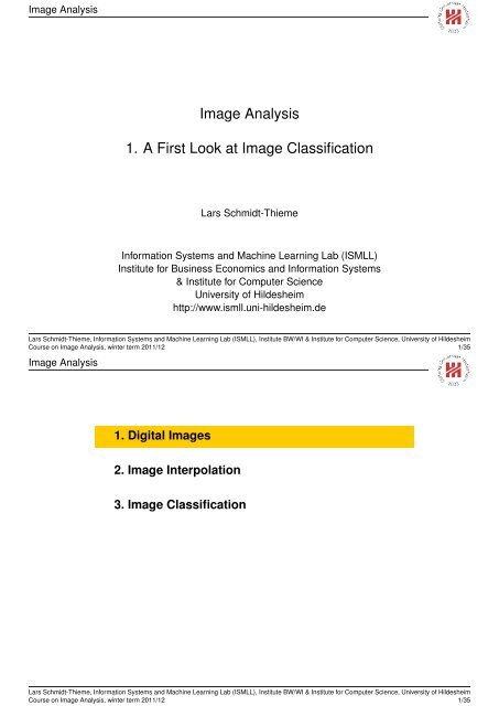
<strong>Image</strong> <strong>Analysis</strong><br />
<strong>Image</strong> <strong>Analysis</strong><br />
<strong>1.</strong> A <strong>First</strong> <strong>Look</strong> <strong>at</strong> <strong>Image</strong> Classific<strong>at</strong>ion<br />
Lars Schmidt-Thieme<br />
Inform<strong>at</strong>ion Systems and Machine Learning Lab (<strong>ISMLL</strong>)<br />
Institute for Business Economics and Inform<strong>at</strong>ion Systems<br />
& Institute for Computer Science<br />
University of Hildesheim<br />
http://www.ismll.uni-hildesheim.de<br />
Lars Schmidt-Thieme, Inform<strong>at</strong>ion Systems and Machine Learning Lab (<strong>ISMLL</strong>), Institute BW/WI & Institute for Computer Science, University of Hildesheim<br />
Course on <strong>Image</strong> <strong>Analysis</strong>, winter term 2011/12 1/35<br />
<strong>Image</strong> <strong>Analysis</strong><br />
<strong>1.</strong> Digital <strong>Image</strong>s<br />
2. <strong>Image</strong> Interpol<strong>at</strong>ion<br />
3. <strong>Image</strong> Classific<strong>at</strong>ion<br />
Lars Schmidt-Thieme, Inform<strong>at</strong>ion Systems and Machine Learning Lab (<strong>ISMLL</strong>), Institute BW/WI & Institute for Computer Science, University of Hildesheim<br />
Course on <strong>Image</strong> <strong>Analysis</strong>, winter term 2011/12 1/35
<strong>Image</strong> <strong>Analysis</strong> / <strong>1.</strong> Digital <strong>Image</strong>s<br />
Perspective Projection<br />
Y<br />
(x,y,z)<br />
X<br />
(u,v)<br />
v<br />
u<br />
y<br />
x<br />
f<br />
Z<br />
image pane<br />
Lars Schmidt-Thieme, Inform<strong>at</strong>ion Systems and Machine Learning Lab (<strong>ISMLL</strong>), Institute BW/WI & Institute for Computer Science, University of Hildesheim<br />
Course on <strong>Image</strong> <strong>Analysis</strong>, winter term 2011/12 1/35<br />
<strong>Image</strong> <strong>Analysis</strong> / <strong>1.</strong> Digital <strong>Image</strong>s<br />
Perspective Projection<br />
Y<br />
(x,y,z)<br />
X<br />
(u,v)<br />
v<br />
u<br />
y<br />
x<br />
f<br />
Z<br />
image pane<br />
Two-dimensional images often are projections from 3D scenes:<br />
X = (x, y, z)<br />
u = (u, v)<br />
u = x f<br />
z , v = y f<br />
z<br />
co-ordin<strong>at</strong>es in 3D scene<br />
co-ordin<strong>at</strong>es in 2D image pane<br />
transform<strong>at</strong>ion<br />
f is called focal length.<br />
Lars Schmidt-Thieme, Inform<strong>at</strong>ion Systems and Machine Learning Lab (<strong>ISMLL</strong>), Institute BW/WI & Institute for Computer Science, University of Hildesheim<br />
Course on <strong>Image</strong> <strong>Analysis</strong>, winter term 2011/12 1/35
<strong>Image</strong> <strong>Analysis</strong> / <strong>1.</strong> Digital <strong>Image</strong>s<br />
<strong>Image</strong> Functions<br />
<strong>Image</strong>s are described by image functions, th<strong>at</strong> for each<br />
co-ordin<strong>at</strong>e tuple provide an intensity value (also: brightness<br />
value).<br />
2D Continuous image function:<br />
where<br />
x : X × Y → I<br />
– X, Y are intervalls in R defining the<br />
ranges of the co-ordin<strong>at</strong>e values and<br />
– I defines the intensity of the points.<br />
discrete / digital / raster 2d image<br />
function:<br />
where<br />
u : U × V → J<br />
– U := {0, 1, 2, . . . , n − 1} and<br />
V := {0, 1, 2, . . . , m − 1} are discrete<br />
co-ordin<strong>at</strong>e ranges and<br />
– J defines discrete intensities of<br />
pixels.<br />
Lars Schmidt-Thieme, Inform<strong>at</strong>ion Systems and Machine Learning Lab (<strong>ISMLL</strong>), Institute BW/WI & Institute for Computer Science, University of Hildesheim<br />
Course on <strong>Image</strong> <strong>Analysis</strong>, winter term 2011/12 2/35<br />
<strong>Image</strong> <strong>Analysis</strong> / <strong>1.</strong> Digital <strong>Image</strong>s<br />
Intensities<br />
Different types of images are modelled by different intensity<br />
ranges:<br />
Binary images:<br />
I := {0, 1}<br />
i.e., each pixel can be either white (1) or black (0).<br />
Gray-level images:<br />
I := [0, I max ] or J := {0, 1, . . . , I max }<br />
i.e., each pixel can have a scalar grey-level intensity value<br />
between white (I max ) and black (0).<br />
Lars Schmidt-Thieme, Inform<strong>at</strong>ion Systems and Machine Learning Lab (<strong>ISMLL</strong>), Institute BW/WI & Institute for Computer Science, University of Hildesheim<br />
Course on <strong>Image</strong> <strong>Analysis</strong>, winter term 2011/12 3/35
<strong>Image</strong> <strong>Analysis</strong> / <strong>1.</strong> Digital <strong>Image</strong>s<br />
Intensities<br />
binary image:<br />
gray-level image (256 different levels)<br />
Lars Schmidt-Thieme, Inform<strong>at</strong>ion Systems and Machine Learning Lab (<strong>ISMLL</strong>), Institute BW/WI & Institute for Computer Science, University of Hildesheim<br />
Course on <strong>Image</strong> <strong>Analysis</strong>, winter term 2011/12 4/35<br />
<strong>Image</strong> <strong>Analysis</strong> / <strong>1.</strong> Digital <strong>Image</strong>s<br />
Intensities / Color<br />
Color images:<br />
I := [0, I max ] 3 or J := {0, 1, . . . , I max } 3<br />
i.e., each pixel is described by 3 different intensity values<br />
between full intensity (I max ) and no intensity (0) for three different<br />
color components, e.g., red, green, blue (RGB color model).<br />
These different values are called channels.<br />
RGB cube:<br />
[from http://imageprocessing.wordpress.com/2008/03/14/image-segment<strong>at</strong>ion/]<br />
Lars Schmidt-Thieme, Inform<strong>at</strong>ion Systems and Machine Learning Lab (<strong>ISMLL</strong>), Institute BW/WI & Institute for Computer Science, University of Hildesheim<br />
Course on <strong>Image</strong> <strong>Analysis</strong>, winter term 2011/12 5/35
<strong>Image</strong> <strong>Analysis</strong> / <strong>1.</strong> Digital <strong>Image</strong>s<br />
Intensities / Color<br />
Lars Schmidt-Thieme, Inform<strong>at</strong>ion Systems and Machine Learning Lab (<strong>ISMLL</strong>), Institute BW/WI & Institute for Computer Science, University of Hildesheim<br />
Course on <strong>Image</strong> <strong>Analysis</strong>, winter term 2011/12 6/35<br />
<strong>Image</strong> <strong>Analysis</strong> / <strong>1.</strong> Digital <strong>Image</strong>s<br />
More Color Models<br />
• RGB (red, green, blue) is an additive color model.<br />
• CMY (Cyan, Magenta, Yellow) is the corresponding<br />
subtractive color model (used in printing; CMYK = CMY plus<br />
black).<br />
• HSV (Hue, S<strong>at</strong>ur<strong>at</strong>ion, Value)<br />
[http://en.wikipedia.org/wiki/HSL_and_HSV]<br />
Lars Schmidt-Thieme, Inform<strong>at</strong>ion Systems and Machine Learning Lab (<strong>ISMLL</strong>), Institute BW/WI & Institute for Computer Science, University of Hildesheim<br />
Course on <strong>Image</strong> <strong>Analysis</strong>, winter term 2011/12 7/35
<strong>Image</strong> <strong>Analysis</strong> / <strong>1.</strong> Digital <strong>Image</strong>s<br />
From RGB to HSV<br />
Let (r, g, b) be the three components of a RGB color pixel and<br />
max :=max{r, g, b}<br />
min :=min{r, g, b}<br />
⎧<br />
0, if max = min<br />
⎪⎨<br />
60 o g−b ·<br />
h :=<br />
max−min + 0o , if max = r<br />
60<br />
⎪⎩<br />
o b−r ·<br />
max−min + 120o , if max = g<br />
60 o r−g ·<br />
max−min + 240o , if max = b<br />
{ 0, if max = 0<br />
s := max−min<br />
max<br />
, else<br />
v :=max<br />
– Hue h describes the dominant primary color<br />
(0-120 redish, 120-240 greenish, 240-360 blueish),<br />
– S<strong>at</strong>ur<strong>at</strong>ion s describes the rel<strong>at</strong>ive intensity of the dominant<br />
primary color over the least dominant primary color,<br />
– Value v describes the absolute intensity of the dominant<br />
primary color.<br />
Lars Schmidt-Thieme, Inform<strong>at</strong>ion Systems and Machine Learning Lab (<strong>ISMLL</strong>), Institute BW/WI & Institute for Computer Science, University of Hildesheim<br />
Course on <strong>Image</strong> <strong>Analysis</strong>, winter term 2011/12 8/35<br />
<strong>Image</strong> <strong>Analysis</strong> / <strong>1.</strong> Digital <strong>Image</strong>s<br />
Palette images / Indexed images<br />
A palette image is a special way to store intensity values:<br />
• the intensity value is an index into a lookup table,<br />
• the lookup table stores the map from intensity indices to<br />
some intensity represent<strong>at</strong>ion, e.g., RGB, HSV, gray-levels etc.<br />
Many raster image form<strong>at</strong>s such as TIFF, PNG and GIF can store<br />
images as palette images.<br />
Lars Schmidt-Thieme, Inform<strong>at</strong>ion Systems and Machine Learning Lab (<strong>ISMLL</strong>), Institute BW/WI & Institute for Computer Science, University of Hildesheim<br />
Course on <strong>Image</strong> <strong>Analysis</strong>, winter term 2011/12 9/35
<strong>Image</strong> <strong>Analysis</strong> / <strong>1.</strong> Digital <strong>Image</strong>s<br />
From Color to Gray-levels to Binary<br />
A color image can be converted into a gray-level image simply by<br />
averaging the intensities of the three channels:<br />
X gray (x, y) := X(x, y) 1 + X(x, y) 2 + X(x, y) 3<br />
3<br />
A gray-level image can be converted to a binary image by<br />
thresholding:<br />
{ 1, if X(x, y) ≥<br />
X binary Ithreshold<br />
(x, y) :=<br />
0, else<br />
with a given intensity threshold I threshold ∈ I.<br />
Lars Schmidt-Thieme, Inform<strong>at</strong>ion Systems and Machine Learning Lab (<strong>ISMLL</strong>), Institute BW/WI & Institute for Computer Science, University of Hildesheim<br />
Course on <strong>Image</strong> <strong>Analysis</strong>, winter term 2011/12 10/35<br />
<strong>Image</strong> <strong>Analysis</strong> / <strong>1.</strong> Digital <strong>Image</strong>s<br />
<strong>Image</strong> Digitiz<strong>at</strong>ion<br />
When a continuous image function is processed in a computer, it<br />
needs to be digitized, i.e., represented as raster image. This<br />
involes two aspects:<br />
• sampling:<br />
the intensity of the continuous image is measured <strong>at</strong><br />
sampling points, usually organized in a square grid.<br />
Sampling points usually are called pixels (or image element<br />
or voxels in 3D).<br />
Typical grid sizes are around 512 × 512 (768 × 576 for PAL TV,<br />
640 × 480 for NTSC TV, 1920 × 1080 for HDTV)<br />
• Quantiz<strong>at</strong>ion:<br />
the intensity <strong>at</strong> each pixel is discretized in a given number of<br />
levels.<br />
A typical number of levels is 256 (8 bits; per channel).<br />
A 512 × 512 RGB color image with 256 levels / channel is 768 kB<br />
(uncompressed).<br />
Lars Schmidt-Thieme, Inform<strong>at</strong>ion Systems and Machine Learning Lab (<strong>ISMLL</strong>), Institute BW/WI & Institute for Computer Science, University of Hildesheim<br />
Course on <strong>Image</strong> <strong>Analysis</strong>, winter term 2011/12 11/35
<strong>Image</strong> <strong>Analysis</strong> / <strong>1.</strong> Digital <strong>Image</strong>s<br />
Different Sampling / Sp<strong>at</strong>ial Resolution<br />
Lars Schmidt-Thieme, Inform<strong>at</strong>ion Systems and Machine Learning Lab (<strong>ISMLL</strong>), Institute BW/WI & Institute for Computer Science, University of Hildesheim<br />
Course on <strong>Image</strong> <strong>Analysis</strong>, winter term 2011/12 12/35<br />
<strong>Image</strong> <strong>Analysis</strong> / <strong>1.</strong> Digital <strong>Image</strong>s<br />
Different Quantiz<strong>at</strong>ion / Radiometric Resolution<br />
64 intensity levels:<br />
16 intensity levels:<br />
4 intensity levels:<br />
2 intensity levels:<br />
Lars Schmidt-Thieme, Inform<strong>at</strong>ion Systems and Machine Learning Lab (<strong>ISMLL</strong>), Institute BW/WI & Institute for Computer Science, University of Hildesheim<br />
Course on <strong>Image</strong> <strong>Analysis</strong>, winter term 2011/12 12/35
<strong>Image</strong> <strong>Analysis</strong> / <strong>1.</strong> Digital <strong>Image</strong>s<br />
<strong>Image</strong> Resolution<br />
How well the digitized image describes the continuous original<br />
image, can be described by several types of resolutions:<br />
• sp<strong>at</strong>ial resolution: the distance between two pixels.<br />
• spectral resolution: bandwidth (frequency spectrum)<br />
captured by the light sensor.<br />
• radiometric resolution: number of different gray levels.<br />
• time resolution: interval between two samples in time (for<br />
videos).<br />
Lars Schmidt-Thieme, Inform<strong>at</strong>ion Systems and Machine Learning Lab (<strong>ISMLL</strong>), Institute BW/WI & Institute for Computer Science, University of Hildesheim<br />
Course on <strong>Image</strong> <strong>Analysis</strong>, winter term 2011/12 13/35<br />
<strong>Image</strong> <strong>Analysis</strong><br />
<strong>1.</strong> Digital <strong>Image</strong>s<br />
2. <strong>Image</strong> Interpol<strong>at</strong>ion<br />
3. <strong>Image</strong> Classific<strong>at</strong>ion<br />
Lars Schmidt-Thieme, Inform<strong>at</strong>ion Systems and Machine Learning Lab (<strong>ISMLL</strong>), Institute BW/WI & Institute for Computer Science, University of Hildesheim<br />
Course on <strong>Image</strong> <strong>Analysis</strong>, winter term 2011/12 14/35
<strong>Image</strong> <strong>Analysis</strong> / 2. <strong>Image</strong> Interpol<strong>at</strong>ion<br />
Interpol<strong>at</strong>ion<br />
Let f be a raster image of size n × m.<br />
We look for a scaled represent<strong>at</strong>ion f ′ of size n ′ × m ′ .<br />
The corresponding co-ordin<strong>at</strong>es of pixel (x ′ , y ′ ) in image f are<br />
⎛ ⎞<br />
T −1 (x ′ , y ′ ) :=<br />
⎜<br />
⎝<br />
x ′ (n−1)<br />
(n ′ −1)<br />
y ′ (m−1)<br />
(m ′ −1)<br />
Lars Schmidt-Thieme, Inform<strong>at</strong>ion Systems and Machine Learning Lab (<strong>ISMLL</strong>), Institute BW/WI & Institute for Computer Science, University of Hildesheim<br />
Course on <strong>Image</strong> <strong>Analysis</strong>, winter term 2011/12 14/35<br />
<strong>Image</strong> <strong>Analysis</strong> / 2. <strong>Image</strong> Interpol<strong>at</strong>ion<br />
Interpol<strong>at</strong>ion<br />
⎟<br />
⎠<br />
Example: n = m = 3, n ′ = m ′ = 4.<br />
The f-co-ordin<strong>at</strong>es of (2, 1) are<br />
As this is not a gridpoint of f,<br />
there is no measured intensity!<br />
the intensity has to be<br />
interpol<strong>at</strong>ed.<br />
T −1 (2, 1) = (<strong>1.</strong>33, 0.66)<br />
Lars Schmidt-Thieme, Inform<strong>at</strong>ion Systems and Machine Learning Lab (<strong>ISMLL</strong>), Institute BW/WI & Institute for Computer Science, University of Hildesheim<br />
Course on <strong>Image</strong> <strong>Analysis</strong>, winter term 2011/12 15/35
<strong>Image</strong> <strong>Analysis</strong> / 2. <strong>Image</strong> Interpol<strong>at</strong>ion<br />
Nearest-Neighbor Interpol<strong>at</strong>ion<br />
The intensity could be estim<strong>at</strong>ed by the intensity of its nearest<br />
neighbor:<br />
f ′ (x ′ , y ′ ) := f(round(T −1 (x ′ , y ′ )))<br />
Example:<br />
f ′ (2, 1) := f(round(T −1 (x, y))) = f(round(<strong>1.</strong>33, 0.66)) = f(1, 1)<br />
Lars Schmidt-Thieme, Inform<strong>at</strong>ion Systems and Machine Learning Lab (<strong>ISMLL</strong>), Institute BW/WI & Institute for Computer Science, University of Hildesheim<br />
Course on <strong>Image</strong> <strong>Analysis</strong>, winter term 2011/12 16/35<br />
<strong>Image</strong> <strong>Analysis</strong> / 2. <strong>Image</strong> Interpol<strong>at</strong>ion<br />
Bi-linear Interpol<strong>at</strong>ion<br />
A better estim<strong>at</strong>ion uses all four neighbors and the distances:<br />
with<br />
f ′ (x ′ , y ′ ) :=(1 − a) (1 − b) f(x, y) + a (1 − b) f(x + 1, y)<br />
+(1 − a) b f(x, y + 1) + a b f(x + 1, y + 1)<br />
(x, y) := floor(T −1 (x ′ , y ′ ))<br />
a := T −1 (x ′ , y ′ ) 1 − x<br />
b := T −1 (x ′ , y ′ ) 2 − y<br />
Example:<br />
f ′ (2, 1) := 0.66·0.33·f(1, 0)+0.33·0.33·f(2, 0)+0.66·0.66f(1, 1)+0.33·0.66·f(2, 1)<br />
a<br />
b<br />
Lars Schmidt-Thieme, Inform<strong>at</strong>ion Systems and Machine Learning Lab (<strong>ISMLL</strong>), Institute BW/WI & Institute for Computer Science, University of Hildesheim<br />
Course on <strong>Image</strong> <strong>Analysis</strong>, winter term 2011/12 17/35
<strong>Image</strong> <strong>Analysis</strong> / 2. <strong>Image</strong> Interpol<strong>at</strong>ion<br />
More Interpol<strong>at</strong>ion Methods<br />
There are more complex interpol<strong>at</strong>ion methods:<br />
• bi-cubic interpol<strong>at</strong>ion: uses 16 neighboring points and a<br />
bi-cubic polynomial surface.<br />
• area interpol<strong>at</strong>ion: uses all the points covered by a target<br />
pixel.<br />
Nearest-neighbor interpol<strong>at</strong>ion may introduce step-like<br />
appearances, esp. for straight lines.<br />
Linear interpol<strong>at</strong>ion can cause blur due to the averaging.<br />
Lars Schmidt-Thieme, Inform<strong>at</strong>ion Systems and Machine Learning Lab (<strong>ISMLL</strong>), Institute BW/WI & Institute for Computer Science, University of Hildesheim<br />
Course on <strong>Image</strong> <strong>Analysis</strong>, winter term 2011/12 18/35<br />
<strong>Image</strong> <strong>Analysis</strong> / 2. <strong>Image</strong> Interpol<strong>at</strong>ion<br />
Interpol<strong>at</strong>ion / Moire Effect<br />
The next two slides show an original image (bricks.jpg, 622 × 756)<br />
and downsamples of size 205 × 250 by four different methods:<br />
• nearest neighbor interpol<strong>at</strong>ion (upper left)<br />
• bi-linear interpol<strong>at</strong>ion (upper right)<br />
• bi-cubic interpol<strong>at</strong>ion (lower left)<br />
• area interpol<strong>at</strong>ion (lower right)<br />
Lars Schmidt-Thieme, Inform<strong>at</strong>ion Systems and Machine Learning Lab (<strong>ISMLL</strong>), Institute BW/WI & Institute for Computer Science, University of Hildesheim<br />
Course on <strong>Image</strong> <strong>Analysis</strong>, winter term 2011/12 19/35
<strong>Image</strong> <strong>Analysis</strong> / 2. <strong>Image</strong> Interpol<strong>at</strong>ion<br />
[http://en.wikipedia.org/wiki/Moire]<br />
Lars Schmidt-Thieme, Inform<strong>at</strong>ion Systems and Machine Learning Lab (<strong>ISMLL</strong>), Institute BW/WI & Institute for Computer Science, University of Hildesheim<br />
Course on <strong>Image</strong> <strong>Analysis</strong>, winter term 2011/12 20/35<br />
<strong>Image</strong> <strong>Analysis</strong> / 2. <strong>Image</strong> Interpol<strong>at</strong>ion<br />
Interpol<strong>at</strong>ion / Example<br />
Lars Schmidt-Thieme, Inform<strong>at</strong>ion Systems and Machine Learning Lab (<strong>ISMLL</strong>), Institute BW/WI & Institute for Computer Science, University of Hildesheim<br />
Course on <strong>Image</strong> <strong>Analysis</strong>, winter term 2011/12 21/35
<strong>Image</strong> <strong>Analysis</strong> / 2. <strong>Image</strong> Interpol<strong>at</strong>ion<br />
Interpol<strong>at</strong>ion / Example 2 (1/2)<br />
nearest neighbor:<br />
bi-linear:<br />
Lars Schmidt-Thieme, Inform<strong>at</strong>ion Systems and Machine Learning Lab (<strong>ISMLL</strong>), Institute BW/WI & Institute for Computer Science, University of Hildesheim<br />
Course on <strong>Image</strong> <strong>Analysis</strong>, winter term 2011/12 22/35<br />
<strong>Image</strong> <strong>Analysis</strong> / 2. <strong>Image</strong> Interpol<strong>at</strong>ion<br />
Interpol<strong>at</strong>ion / Example 2 (2/2)<br />
bi-linear:<br />
bi-cubic:<br />
Lars Schmidt-Thieme, Inform<strong>at</strong>ion Systems and Machine Learning Lab (<strong>ISMLL</strong>), Institute BW/WI & Institute for Computer Science, University of Hildesheim<br />
Course on <strong>Image</strong> <strong>Analysis</strong>, winter term 2011/12 23/35
<strong>Image</strong> <strong>Analysis</strong><br />
<strong>1.</strong> Digital <strong>Image</strong>s<br />
2. <strong>Image</strong> Interpol<strong>at</strong>ion<br />
3. <strong>Image</strong> Classific<strong>at</strong>ion<br />
Lars Schmidt-Thieme, Inform<strong>at</strong>ion Systems and Machine Learning Lab (<strong>ISMLL</strong>), Institute BW/WI & Institute for Computer Science, University of Hildesheim<br />
Course on <strong>Image</strong> <strong>Analysis</strong>, winter term 2011/12 24/35<br />
<strong>Image</strong> <strong>Analysis</strong> / 3. <strong>Image</strong> Classific<strong>at</strong>ion<br />
A <strong>First</strong> <strong>Look</strong> <strong>at</strong> <strong>Image</strong> Classific<strong>at</strong>ion<br />
Given<br />
– images and<br />
– some (global) annot<strong>at</strong>ion,<br />
e.g., if the image shows a person or<br />
not,<br />
try to learn the annot<strong>at</strong>ed concept,<br />
so th<strong>at</strong> the annot<strong>at</strong>ion can be done<br />
autom<strong>at</strong>ically in future.<br />
Useful for<br />
• image retrieval<br />
(search by keyword/tag).<br />
• many applic<strong>at</strong>ions<br />
(e.g., sort tom<strong>at</strong>o plants).<br />
image<br />
person?<br />
no<br />
yes<br />
no<br />
yes<br />
?<br />
Lars Schmidt-Thieme, Inform<strong>at</strong>ion Systems and Machine Learning Lab (<strong>ISMLL</strong>), Institute BW/WI & Institute for Computer Science, University of Hildesheim<br />
Course on <strong>Image</strong> <strong>Analysis</strong>, winter term 2011/12 24/35
<strong>Image</strong> <strong>Analysis</strong> / 3. <strong>Image</strong> Classific<strong>at</strong>ion<br />
How to Learn? / Trainig D<strong>at</strong>a<br />
To predict if an entity belongs to a specific class, a machine<br />
needs the following components:<br />
<strong>1.</strong> training d<strong>at</strong>a (x j , y j ) j=1,...,N consisting of N pairs<br />
(x, y) ∈ X × Y where<br />
– x = (x i ) i=1,...,n are the predictor variables th<strong>at</strong> describe an<br />
entity and<br />
– y is the observed class label, also called target variable,<br />
here for simplicity:<br />
y = 1: entity belongs to the class,<br />
y = 0: entity does not belong to the class.<br />
Lars Schmidt-Thieme, Inform<strong>at</strong>ion Systems and Machine Learning Lab (<strong>ISMLL</strong>), Institute BW/WI & Institute for Computer Science, University of Hildesheim<br />
Course on <strong>Image</strong> <strong>Analysis</strong>, winter term 2011/12 25/35<br />
<strong>Image</strong> <strong>Analysis</strong> / 3. <strong>Image</strong> Classific<strong>at</strong>ion<br />
How to Learn? / Training D<strong>at</strong>a<br />
Entities are described by two predictor variables<br />
(horizontal & vertical axis).<br />
Classes are depicted by colors: green = 1, red = 0.<br />
Lars Schmidt-Thieme, Inform<strong>at</strong>ion Systems and Machine Learning Lab (<strong>ISMLL</strong>), Institute BW/WI & Institute for Computer Science, University of Hildesheim<br />
Course on <strong>Image</strong> <strong>Analysis</strong>, winter term 2011/12 26/35
<strong>Image</strong> <strong>Analysis</strong> / 3. <strong>Image</strong> Classific<strong>at</strong>ion<br />
How to Learn? / Models<br />
To predict if an entity belongs to a specific class, a machine<br />
needs the following components:<br />
2. a model<br />
ŷ : X → Y<br />
th<strong>at</strong> describes how the target variable Y depends on the<br />
predictor variables X.<br />
Example: the linear support vector machine (a specific<br />
model) decides if an entity x belongs to a class or not via<br />
n∑<br />
ŷ(x) = 1 :⇐⇒ a i x i ≥ 0<br />
where<br />
– a = (a i ) i=1,...,n are parameters of the model th<strong>at</strong> need to be<br />
learned and<br />
– ŷ denotes the class label predicted by the model.<br />
i=1<br />
Lars Schmidt-Thieme, Inform<strong>at</strong>ion Systems and Machine Learning Lab (<strong>ISMLL</strong>), Institute BW/WI & Institute for Computer Science, University of Hildesheim<br />
Course on <strong>Image</strong> <strong>Analysis</strong>, winter term 2011/12 27/35<br />
<strong>Image</strong> <strong>Analysis</strong> / 3. <strong>Image</strong> Classific<strong>at</strong>ion<br />
How to Learn? / Models / SVM<br />
separ<strong>at</strong>ing<br />
hyperplane<br />
Lars Schmidt-Thieme, Inform<strong>at</strong>ion Systems and Machine Learning Lab (<strong>ISMLL</strong>), Institute BW/WI & Institute for Computer Science, University of Hildesheim<br />
Course on <strong>Image</strong> <strong>Analysis</strong>, winter term 2011/12 27/35
<strong>Image</strong> <strong>Analysis</strong> / 3. <strong>Image</strong> Classific<strong>at</strong>ion<br />
How to Learn? / Models / SVM<br />
normal a<br />
separ<strong>at</strong>ing<br />
hyperplane<br />
The points on the hyperplane are described by 〈a, x〉 = 0.<br />
For points on the side pointed to by the normal, 〈a, x〉 > 0.<br />
Lars Schmidt-Thieme, Inform<strong>at</strong>ion Systems and Machine Learning Lab (<strong>ISMLL</strong>), Institute BW/WI & Institute for Computer Science, University of Hildesheim<br />
Course on <strong>Image</strong> <strong>Analysis</strong>, winter term 2011/12 27/35<br />
<strong>Image</strong> <strong>Analysis</strong> / 3. <strong>Image</strong> Classific<strong>at</strong>ion<br />
How to Learn? / Error Measures & Learning Algorithms<br />
To predict if an entity belongs to a specific class, a machine<br />
needs the following components:<br />
3. a learning algorithm th<strong>at</strong> estim<strong>at</strong>es the parameters a from<br />
the training d<strong>at</strong>a, i.e., chooses the parameters such th<strong>at</strong> the<br />
error of the classifier is small.<br />
Example: for a binary classific<strong>at</strong>ion problem, accurracy is a<br />
simple error measure:<br />
accurray(ŷ, (x j , y j ) j=1,...,N ) := 1 N∑<br />
I(ŷ(x j ) = y j )<br />
N<br />
where<br />
j=1<br />
{ 1, if x is true<br />
I(x) :=<br />
0, else<br />
Lars Schmidt-Thieme, Inform<strong>at</strong>ion Systems and Machine Learning Lab (<strong>ISMLL</strong>), Institute BW/WI & Institute for Computer Science, University of Hildesheim<br />
Course on <strong>Image</strong> <strong>Analysis</strong>, winter term 2011/12 28/35
<strong>Image</strong> <strong>Analysis</strong> / 3. <strong>Image</strong> Classific<strong>at</strong>ion<br />
How to Learn? / Models / SVM<br />
normal a<br />
separ<strong>at</strong>ing<br />
hyperplane<br />
Among all possible hyperplanes, the SVM searches for the one<br />
with the maximal margin.<br />
Lars Schmidt-Thieme, Inform<strong>at</strong>ion Systems and Machine Learning Lab (<strong>ISMLL</strong>), Institute BW/WI & Institute for Computer Science, University of Hildesheim<br />
Course on <strong>Image</strong> <strong>Analysis</strong>, winter term 2011/12 28/35<br />
<strong>Image</strong> <strong>Analysis</strong> / 3. <strong>Image</strong> Classific<strong>at</strong>ion<br />
How to Learn? / Models / SVM<br />
normal a<br />
separ<strong>at</strong>ing<br />
hyperplane<br />
Lars Schmidt-Thieme, Inform<strong>at</strong>ion Systems and Machine Learning Lab (<strong>ISMLL</strong>), Institute BW/WI & Institute for Computer Science, University of Hildesheim<br />
Course on <strong>Image</strong> <strong>Analysis</strong>, winter term 2011/12 28/35
<strong>Image</strong> <strong>Analysis</strong> / 3. <strong>Image</strong> Classific<strong>at</strong>ion<br />
How to Describe an <strong>Image</strong>? (1/3)<br />
To apply machine learning techniques, entities (usually)<br />
have to be described by predictor variables having<br />
numerical values.<br />
As entities are compared via their predictor variables, all<br />
entities need to have the same predictor variables.<br />
Wh<strong>at</strong> can we do in the case of images?<br />
480 × 320 pixels a 3 channels. 320 × 480 pixels a 3 channels.<br />
Lars Schmidt-Thieme, Inform<strong>at</strong>ion Systems and Machine Learning Lab (<strong>ISMLL</strong>), Institute BW/WI & Institute for Computer Science, University of Hildesheim<br />
Course on <strong>Image</strong> <strong>Analysis</strong>, winter term 2011/12 29/35<br />
<strong>Image</strong> <strong>Analysis</strong> / 3. <strong>Image</strong> Classific<strong>at</strong>ion<br />
How to Describe an <strong>Image</strong>? (2/3)<br />
Idea:<br />
<strong>1.</strong> Resize image to resolution k × k.<br />
2. Compare pixelwise.<br />
original image: resize to resolution 1 × 1:<br />
original image: resize to resolution 2 × 2:<br />
Lars Schmidt-Thieme, Inform<strong>at</strong>ion Systems and Machine Learning Lab (<strong>ISMLL</strong>), Institute BW/WI & Institute for Computer Science, University of Hildesheim<br />
Course on <strong>Image</strong> <strong>Analysis</strong>, winter term 2011/12 30/35
<strong>Image</strong> <strong>Analysis</strong> / 3. <strong>Image</strong> Classific<strong>at</strong>ion<br />
How to Describe an <strong>Image</strong>? (3/3)<br />
image fe<strong>at</strong>ures person?<br />
237 245 245 no<br />
238 222 209 yes<br />
64 65 61 no<br />
162 157 159 yes<br />
114 138 144 ?<br />
Lars Schmidt-Thieme, Inform<strong>at</strong>ion Systems and Machine Learning Lab (<strong>ISMLL</strong>), Institute BW/WI & Institute for Computer Science, University of Hildesheim<br />
Course on <strong>Image</strong> <strong>Analysis</strong>, winter term 2011/12 31/35<br />
<strong>Image</strong> <strong>Analysis</strong> / 3. <strong>Image</strong> Classific<strong>at</strong>ion<br />
A Trivial Classifier as Baseline<br />
Assume you do not have any inform<strong>at</strong>ion about the image to<br />
classify, but still you have to make a decision.<br />
You only have inform<strong>at</strong>ion about the class frequencies,<br />
e.g., you know th<strong>at</strong> 67% of all images in the training d<strong>at</strong>a belong<br />
to the class persons.<br />
Which class, person or not person, would you predict?<br />
Lars Schmidt-Thieme, Inform<strong>at</strong>ion Systems and Machine Learning Lab (<strong>ISMLL</strong>), Institute BW/WI & Institute for Computer Science, University of Hildesheim<br />
Course on <strong>Image</strong> <strong>Analysis</strong>, winter term 2011/12 32/35
<strong>Image</strong> <strong>Analysis</strong> / 3. <strong>Image</strong> Classific<strong>at</strong>ion<br />
A Trivial Classifier as Baseline<br />
Assume you do not have any inform<strong>at</strong>ion about the image to<br />
classify, but still you have to make a decision.<br />
You only have inform<strong>at</strong>ion about the class frequencies,<br />
e.g., you know th<strong>at</strong> 67% of all images in the training d<strong>at</strong>a belong<br />
to the class persons.<br />
Which class, person or not person, would you predict?<br />
Person, as it is the majority class:<br />
ŷ majority := argmax y∈Y ˆp(y),<br />
ˆp(y) := |{j ∈ {1, . . . , N} | y j = y}|/N<br />
with expected accurracy ˆp(ŷ majority ) = 0.67.<br />
Lars Schmidt-Thieme, Inform<strong>at</strong>ion Systems and Machine Learning Lab (<strong>ISMLL</strong>), Institute BW/WI & Institute for Computer Science, University of Hildesheim<br />
Course on <strong>Image</strong> <strong>Analysis</strong>, winter term 2011/12 32/35<br />
<strong>Image</strong> <strong>Analysis</strong> / 3. <strong>Image</strong> Classific<strong>at</strong>ion<br />
<strong>Image</strong> Classific<strong>at</strong>ion / Example<br />
sky<br />
accuracy<br />
0.60 0.65 0.70 0.75 0.80 0.85 0.90<br />
●<br />
●<br />
●<br />
●<br />
● ● ● ● ● ● ●<br />
●<br />
●<br />
●<br />
●<br />
●<br />
majority class<br />
svm<br />
1 2 3 4 5 6 7<br />
resolution<br />
[D<strong>at</strong>a from <strong>Image</strong>Clef 2008, vcdt, random 50:50 split, hyperparameter C optimized on train]<br />
Lars Schmidt-Thieme, Inform<strong>at</strong>ion Systems and Machine Learning Lab (<strong>ISMLL</strong>), Institute BW/WI & Institute for Computer Science, University of Hildesheim<br />
Course on <strong>Image</strong> <strong>Analysis</strong>, winter term 2011/12 33/35
<strong>Image</strong> <strong>Analysis</strong> / 3. <strong>Image</strong> Classific<strong>at</strong>ion<br />
<strong>Image</strong> Classific<strong>at</strong>ion / Example<br />
person<br />
accuracy<br />
0.56 0.57 0.58 0.59 0.60 0.61 0.62<br />
●<br />
●<br />
●<br />
●<br />
●<br />
●<br />
majority class<br />
svm<br />
●<br />
● ● ● ● ● ● ●<br />
●<br />
1 2 3 4 5 6 7<br />
resolution<br />
[D<strong>at</strong>a from <strong>Image</strong>Clef 2008, vcdt, random 50:50 split, hyperparameter C optimized on train]<br />
Lars Schmidt-Thieme, Inform<strong>at</strong>ion Systems and Machine Learning Lab (<strong>ISMLL</strong>), Institute BW/WI & Institute for Computer Science, University of Hildesheim<br />
Course on <strong>Image</strong> <strong>Analysis</strong>, winter term 2011/12 34/35<br />
<strong>Image</strong> <strong>Analysis</strong> / 3. <strong>Image</strong> Classific<strong>at</strong>ion<br />
Summary (1/2)<br />
• Digital / raster / discrete images can be understood as<br />
discretiz<strong>at</strong>ions of a continuous image function<br />
– with a given sp<strong>at</strong>ial resolution (width and height in pixels)<br />
and<br />
– with a given intensity resolution<br />
(binary, gray-level, color; number of intensity values).<br />
• Color images are represented by several intensity values of<br />
so-called primary colors per pixel (channels), e.g.,<br />
red–green–blue.<br />
• If images are resized, the intensity values of the new grid have<br />
to be interpol<strong>at</strong>ed from itensity values of pixels nearby in the<br />
old grid (nearest-neighbor; bi-linear; bi-cubic; area).<br />
Lars Schmidt-Thieme, Inform<strong>at</strong>ion Systems and Machine Learning Lab (<strong>ISMLL</strong>), Institute BW/WI & Institute for Computer Science, University of Hildesheim<br />
Course on <strong>Image</strong> <strong>Analysis</strong>, winter term 2011/12 35/35
<strong>Image</strong> <strong>Analysis</strong> / 3. <strong>Image</strong> Classific<strong>at</strong>ion<br />
Summary (2/2)<br />
• In image classific<strong>at</strong>ion a model such as a Support Vector<br />
Machine (SVM) is build from training d<strong>at</strong>a. The model can be<br />
applied to test d<strong>at</strong>a to predict unknown class labels.<br />
• Renderings in small grids (1 × 1 to 10 × 10) can be used as<br />
primitive fe<strong>at</strong>ures for image classific<strong>at</strong>ion.<br />
Lars Schmidt-Thieme, Inform<strong>at</strong>ion Systems and Machine Learning Lab (<strong>ISMLL</strong>), Institute BW/WI & Institute for Computer Science, University of Hildesheim<br />
Course on <strong>Image</strong> <strong>Analysis</strong>, winter term 2011/12 35/35