Full Text - Journal of Theoretical and Applied Information Technology

Journal of Theoretical and Applied Information Technology 

20 th November 2013. Vol. 57 No.2 

© 2005 - 2013 JATIT & LLS. All rights reserved . 

ISSN: 1992-8645 www.jatit.org E-ISSN: 1817-3195 

MAMMOGRAM MRI IMAGE SEGMENTATION AND 

CLASSIFICATION 

1 S.PITCHUMANI ANGAYARKANNI*, 2 DR.NADIRA BANU KAMAL, 3 DR.V.THAVAVEL 

1 Assistant Professor, Department of Computer Science, Lady Doak College, Madurai, Tamil Nadu, India. 

2 Head of the Department,Department of M.C.A, TBAK College,Kilakarai,Ramnad,Tamil Nadu,India 

3 Head of the Department, Department of M.C.A., Karunya University, Coimbatore, TamilNadu, India 

E-mail: 1 pitchu_mca@yahoo.com 2 nadira@hotmail.com 3 thavavel@gmail.com 

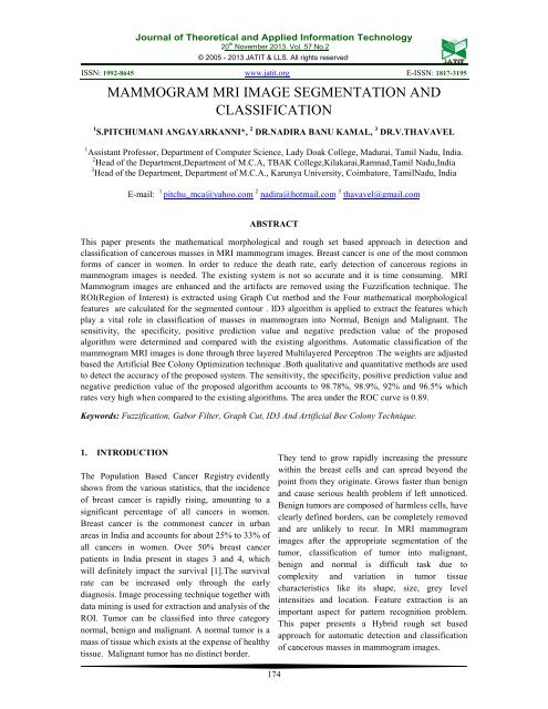
ABSTRACT 

This paper presents the mathematical morphological and rough set based approach in detection and 

classification of cancerous masses in MRI mammogram images. Breast cancer is one of the most common 

forms of cancer in women. In order to reduce the death rate, early detection of cancerous regions in 

mammogram images is needed. The existing system is not so accurate and it is time consuming. MRI 

Mammogram images are enhanced and the artifacts are removed using the Fuzzification technique. The 

ROI(Region of Interest) is extracted using Graph Cut method and the Four mathematical morphological 

features are calculated for the segmented contour . ID3 algorithm is applied to extract the features which 

play a vital role in classification of masses in mammogram into Normal, Benign and Malignant. The 

sensitivity, the specificity, positive prediction value and negative prediction value of the proposed 

algorithm were determined and compared with the existing algorithms. Automatic classification of the 

mammogram MRI images is done through three layered Multilayered Perceptron .The weights are adjusted 

based the Artificial Bee Colony Optimization technique .Both qualitative and quantitative methods are used 

to detect the accuracy of the proposed system. The sensitivity, the specificity, positive prediction value and 

negative prediction value of the proposed algorithm accounts to 98.78%, 98.9%, 92% and 96.5% which 

rates very high when compared to the existing algorithms. The area under the ROC curve is 0.89. 

Keywords: Fuzzification, Gabor Filter, Graph Cut, ID3 And Artificial Bee Colony Technique. 

1. INTRODUCTION 

The Population Based Cancer Registry evidently 

shows from the various statistics, that the incidence 

of breast cancer is rapidly rising, amounting to a 

significant percentage of all cancers in women. 

Breast cancer is the commonest cancer in urban 

areas in India and accounts for about 25% to 33% of 

all cancers in women. Over 50% breast cancer 

patients in India present in stages 3 and 4, which 

will definitely impact the survival [1].The survival 

rate can be increased only through the early 

diagnosis. Image processing technique together with 

data mining is used for extraction and analysis of the 

ROI. Tumor can be classified into three category 

normal, benign and malignant. A normal tumor is a 

mass of tissue which exists at the expense of healthy 

tissue. Malignant tumor has no distinct border. 

They tend to grow rapidly increasing the pressure 

within the breast cells and can spread beyond the 

point from they originate. Grows faster than benign 

and cause serious health problem if left unnoticed. 

Benign tumors are composed of harmless cells, have 

clearly defined borders, can be completely removed 

and are unlikely to recur. In MRI mammogram 

images after the appropriate segmentation of the 

tumor, classification of tumor into malignant, 

benign and normal is difficult task due to 

complexity and variation in tumor tissue 

characteristics like its shape, size, grey level 

intensities and location. Feature extraction is an 

important aspect for pattern recognition problem. 

This paper presents a Hybrid rough set based 

approach for automatic detection and classification 

of cancerous masses in mammogram images. 

174





2. MATERIALS AND METHODS 

The block diagram in Figure 1 clearly depicts the 

methodology of the proposed technique. 

Input 

Image 

Image 

Fuzzificatio 

n 

Membershi 

p 

Modificatio 

Image 

Defuzzification 

Enhanced 

Image 

Figure 2: Fuzzification Technique 

The histogram equalization of the gray levels in the 

original image can be characterized using five 

parameters:( α , ß1,γ, ß2, max) as shown in Figure 3. 

Figure 1: Proposed Methodology 

The data set used for research were taken from 

Mammogram Image Analysis Society(MIAS)[2]. 

The database contains 320 images out of which 206 

are normal images,63 benign and 51 malignant 

cases. 

3. IMAGE ENHANCEMENT AND 

PREPROCESSING USING FUZZY 

HISTOGRAM EQUALIZATION 

Mammogram images are enhanced using histogram 

equalization method. The approach developed by 

Ella Hassanien is implemented for Image 

preprocessing[3]. An image I of size M x N and L 

gray levels can be considered as an array of fuzzy 

singletons, each having a value of membership 

denoting its degree of brightness relative to some 

brightness levels. For an image I, we can write in 

the notation of fuzzy sets [4]: 

I =Uµ mn /g mn m = 1,2,..., M and n = 1,2,..., N, Where 

µ mn its membership function g mn is the intensity of 

(m, n) pixel.The membership function characterizes 

a suitable property of image (e.g. edginess, 

darkness, textural property) and can be defined 

globally for the whole image or locally for its 

segments. In recent years, some researchers have 

applied the concept of fuzziness to develop new 

algorithms for image enhancement [3] . The 

principle of fuzzy enhancement scheme is illustrated 

in Figure 2. 

Figure 3: Histogram Equalization Curve With Α , ß1,Γ, 

ß2, Max 

where the intensity value γ represents the mean 

value of the distribution, α is the minimum, and max 

is the maximum. The aim is to decrease the gray 

levels below ß1, and above ß2. Intensity levels 

between ß1 and γ, and ß2 and γ are stretched in 

opposite directions towards the mean 

γ.The fuzzy 

transformation function for computing the fuzzy 

plane value P is defined as follows: 

α= min; 

β1= (α+ γ) /2; 

β 2= (max + γ) /2; 

γ = mean; max; 

The following fuzzy rules are used for contrast 

enhancement based on Figure (2). 

Rule-1: If α ≤ ui < β1 then P = 2 ( ( ui - α) / ( γ -α ))² 

Rule-2: If β1 ≤ ui < γ then P = 1- 2 ( ( ui – γ )/( γ -α 

))² 

Rule-3: If γ ≤ ui





Set β2 = ( max + mean )/2 

Step-2: Fuzzification 

For all pixels (i,j) within the image Do 

If ((data[i][j]>=min) && (data[i][j]< β1)) 

Compute NewGrayLevel =2*(pow(((data[i][j]- 

min)/(mean- min)),2)) 

If ((data[i][j]> = β1) && (data[i][j] < mean)) 

Compute NewGrayLevel=1-(2*(pow(((data[i][j]- 

mean)/(mean-min)),2))) 

If ((data[i][j]>=mean)&&(data[i][j]< β2)) 

Compute NewGrayLevel=1-(2*(pow(((data[i][j]- 

mean)/(max-mean)),2))) 

If ((data[i][j] >= β2) && (data[i][j]





4. IMAGE SEGMENTATION AND ROI 

EXTRACTION 

The region of Interest ie) the tumor region is 

segmented using the Graph cut method. The main 

purpose of using this method for segmentation is 

that it segments the mammogram into different 

mammographic densities. It is useful for risk 

assessment and quantitative evaluation of density 

changes. Apart from the above advantage it 

produces the contour (closed region) or a convex 

hull which is used for analyzing the morphological 

and novel features of the segmented region. The 

above technique results in efficient formulation of 

attributes which helps in classification of the ROI 

into benign, malignant or normal. Graph Cuts has 

been used in recent years for interactive image 

segmentation[4]. The core ideology of Graph Cuts is 

to map an image onto a network graph, and 

construct an energy function on the labeling, and 

then do energy minimization with dynamic 

optimization techniques. This study proposes a new 

segmentation method using iterated Graph Cuts 

based on multi-scale smoothing. The multi-scale 

method can segment mammographic images with a 

stepwise process from global to local segmentation 

by iterating Graph Cuts. The Graph cut approach 

used by K. Santle Camilus [4] is implemented in 

this paper 

Steps involved in Graph Cut Segmentation are: 

1. Form a graph 

2. Sort the graph edges 

3. Region merging 

A graph G=(V,E) is constructed from the 

mammogram image such that V represent the pixel 

values of the 3*3 image and E the edges defined 

between the neighboring pixels. The weight of any 

edge W(Vi,Vj) is measure of dissimilarity between 

the pixels Vi and Vj. The weight for an edge is by 

means of considering the Euclidian distance 

between the two pixels Vi and Vj. It is represented 

by the equation 

W(Vi,Vj)= 

Vi=(xi,yi) Vj=(xj,yj) 

Eqn.(1) 

Edges are sorted in ascending order of their weights 

such that w(e1)





threshold must be computed based on the IRA and 

other parameters to control the merge operation 

adaptive to the properties of regions. Hence, we 

define a dynamic threshold (DT) for merging 

between two regions R 1 and R 2 as given in the 

following equation 

DT(R1,R2)=Max(IRA(R1)+δ1,IRA(R2)+ δ2) 

Eqn.(6) 

The appropriate selection of the parameters (δ 1 and 

δ 2 ) plays a vital role as it determines the merge of 

regions. Values of these parameters are chosen to 

achieve the following desirable features: (1) when 

more number of regions is present, then the choice 

of the values (of δ 1 and δ 2 ) should favor merging of 

regions; (2) the choice of the values should allow 

the grouping of small regions than large regions. 

The large regions should be merged only when their 

intensity values are more similar; (3) it is preferred 

to have values that are adaptive to the total number 

of regions and the number of vertices in the regions 

that are considered for merge. Hence, the parameters 

δ 1 and δ 2 are defined as 

δ1=C × N R /|R 1 | 

δ2=C × N R /|R 2 | 

Eqn.(7) 

N R - the total number of regions. Initially, N R = |V|, 

the size of the vertices and each merge decreases the 

value of N R by one. |R i | indicates the number of 

vertices in the region “R i .” C is a positive constant 

and is equal to two for the pectoral muscle 

segmentation which is found through experimental 

studies. 

Merge Criterion 

When the pixels of a group have intensity values 

similar to the pixels of the other group, then 

intuitively the calculated IRM between these groups 

should be small. The expected smaller value of the 

IRM to merge these two regions is tested by 

comparing it with the dynamic threshold. Hence, the 

merge criterion, to merge the two regions, R 1 and 

R 2 , is defined as 

Merge(R 1 ,R 2 ), if IRM(R 1 ,R 2 ) 

Eqn(8) 

Figure 5: ROI Extracted Using Graph Cut Method 

5. FEATURE EXTRACTION AND SELECTION 

The main objective of feature extraction and 

selection is to maximize the distinguished 

performance capability of them on interested data 

base. Consideration of significant feature is based 

on discrimination, optimality, reliability and 

independence. In recent years, many kinds of 

features have been reported for breast mass 

classification like texture based features, region 

based features, image structure features, position 

related features, and shape-based features which are 

described and utilized in the CAD systems [4]. In 

our study a set of six novel features based on shape 

characteristics (Novel Feature) proposed by 

Rangaraj M. Rangayyan [5]were extracted from the 

original images which are not applied in breast mass 

classification before and are defined as follows: 

The convex hull which is the smallest convex 

polygon that contains the mass region is displayed. 

Mass’s area is the actual number of pixels in the 

mass region and convex hull’s area is the actual 

number of pixels in the convex hull region. 

178





Compactness(C) 

or Normalized 

circularity 

fractional 

concavity (F cc ) 

Fourier 

descriptors and 

Fourier 

coefficient A 0 

Convexity 

Aspect Ratio 

Solidity 

C is a simple measure of the efficiency of a contour to contain a given area and is 

defined in a normalized form as 1-4πS/D 2 , where D and S are the contour perimeter 

and area 

S=Area= 

where 

Where I(x, y) = 1 if (x ,y) pixel belong to S, zero other case 

D(S)= (X i -X( i-1 )) 2 + (Y i -Y( i-1 )) 2 

is a measure of the portion of the indented length to the total contour length; it is 

computed by taking the cumulative length of the concave segments and dividing it 

by the total length of the contour 

A 0 =1/N 

Where d(i)=√(X(i)-X c ) 2 +(Y(i)-Y c ) 2 

where (xc, yc) are the coordinates of the centroid, (x(i), y(i)) are the coordinates of 

the boundary pixel at the i-th location. 

The measure of convexity of an object is the ratio of the perimeter of the convex 

object to the original perimeter of the object. 

Convexity=convexperimeter/perimeter 

Aspect Ratio is the ratio between height and width of the corresponding object 

Solidity=Area/convexarea 

Circularity 4πS/D 2 

• 

• The information gain is based on the 

The shape features are calculated for the ROI decrease in entropy after a dataset is split on an 

segmented using Graph cut method for 320 images . attribute[7]. 

The results are plotted in an Excel sheet for 

classification using WEKA tool. 

Information Gain(S,A)=Entropy(S)-H(S,A) 

6. FEATURE SELECTION USING ID3 

ALGORITHM 

A mathematical algorithm for building the decision 

tree. Builds the tree from the top down, with no 

backtracking. Information Gain is used to select the 

most useful attribute for classification. 

Where H(S,A)=∑ i (|Si|/|S|).H(Si) 

A takes on value 1 and H(Si) is the entropy of the 

system of subsets Si. 

Entropy 

• A formula to calculate the homogeneity of 

a sample. 

• A completely homogeneous sample has 

entropy of 0. 

• An equally divided sample has entropy of 

1. 

• Entropy(s) = - p+log2 (p+) -p-log2 (p-) for 

a sample of negative and positive elements. 

• The formula for entropy is: 

Information Gain (IG): 

The training data is a set S=s1,s2—of already 

classified samples based on the mathematical 

morphological and novel features. Each sample 

Si=x1,x2 is a vector where x1,x2—represents 

attributes or features of the sample. The training 

data is augmented with a vector C=C1,C2 and C3 

where C1represent benign C2 represents malignant 

and C3 represents normal cases. At each node of the 

tree ID3 chooses one attribute of the data that most 

efficiently splits its set of samples into subsets 

enriched in one class or the other. The criterion is 

the normalized Information Gain that results from 

choosing an attribute for splitting the data. The 

attribute with highest information gain is chosen to 

make decision. 

179





Psudocode: 

Input: Set of 12 =4 Mathematical morphological + 4 

novel feature attributes A1,A2---A12.The class 

labels Ci C1=Benign,C2=Malignant and 

C3=Normal.. Training set S of examples 

Output: Decision tree with set of rules. 

Procedure: 

• All the samples in the list belongs to three different 

classes 

• Create a leaf node for the decision tree saying to 

choose the class. 

• If none of the feature provides IG then ID3 creates a 

decision node higher up the tree using the expected 

value of the class. 

• If instance previously unseen class is encountered 

ID3 creates decision class higher up in the tree using 

expected value. 

• Calculate IG for each attribute 

• Choose attribute A with lowest entropy and Highest 

IG and test this attribute with root. 

• For each possible value v of this attribute 

o Add a new branch below the root corresponding to 

A=v. 

o If v is empty make the new branch a leaf node 

labeled with most common value else 

o Let the new branch be the tree created by ID3 

o 

• End 

The attributes used were the eight parameters with 

the class as benign, malignant and normal. Based on 

the rule derived by testing 320 mammogram images 

the rules are applied in classifying the new cases 

without prior knowledge of whether they are 

benign, malignant or normal. 

Table 2: Nodes Representing The 7 Attributes Cross 

Validation 10 Fold 

=== Detailed Accuracy By Class === 

Class TP Rate FP Rate Precision Recall 

FMS ROC 

Benign 0.595 0.272 0.523 0.595 

0.557 0.677 

Malig 0.121 0.104 0.368 0.121 

0.182 0.542 

Normal 0.678 0.427 0.442 0.678 

0.536 0.637 

Wgt. 0.465 0.268 0.445 0.465 

0.425 0.618 

=== Confusion Matrix === 

a b c = -0.0450 then Class = 

Malignant (62.34 % of 316 examples). 

• Compactness >= -0.0050 then Class = 

Normal (42.29 % of 525 examples) 

ID3 parameters: 

Size before split 200 

Size after split 50 

Max depth of leaves10 

Goodness of split threshold 0.0300 

180





7. MULTILAYER FEED FORWARD NEURAL 

NETWORK (MLN) OPTIMIZED BY 

ARTIFICIAL BEE COLONY OPTIMIZATION 

TECHNIQUE: 

Artificial bee colony algorithm(ABC) was proposed 

for optimization , classification and neural network 

problem solution based on the intelligent foraging 

behavior of honey bee . ABC is more powerful and 

most robust on multimodal functions. It provides 

solution in organized form by dividing the bee 

objects into different tasks such as employed bees, 

onlooker bees and scout bees. It finds global 

optimization results, optimal weight values by bee 

agents. Successfully trained MLN improves the 

classification precision of MRI mammogram images 

into benign, malignant and normal cases. 

The ANN is the best method for pattern recognition. 

The seven attribute values together with the class 

are fed as input to the eight neurons at the input 

layer. The hidden layer has sixteen neurons or 

nodes. The output layer has one node. The error rate 

is calculated by subtracting the actual output with 

the desired output value. The evaluation of the food 

sources that are discovered by the randomly 

generated populations is done through the backpropagation 

procedure. Now after completion of the 

first cycle the performance of each solution is kept 

in an index. In order to generate the population of 

back-propagation, the weight must be created, and 

each value of the weight matrix for every layer is 

randomly generated within the range of [1,0]. Each 

set of weight and bias is used to create one element 

in a whole population. The size of the population in 

the proposed method is fixed to N. 

The classifier employed in this paper is a three-layer 

Back propagation neural network. The Back 

propagation neural network optimizes the net for 

correct responses to the training input data set. More 

than one hidden layer may be beneficial for some 

applications, but one hidden layer is sufficient if 

enough hidden neurons are used. Initially the 

attributes values (rules) from the Mathematical 

morphological and novel approach analysis method 

which plays a vital role in classification between 

benign, malignant and normal cases extracted from 

the ID3 algorithm are normalized between [0,1]. 

That is each value in the feature set is divided by the 

maximum value from the set. These normalized 

values are assigned to the input neurons. The 

number of hidden neurons is equal to the number of 

input neurons and only one output neuron. 

The procedure employed by Habib Shah in his work 

was implemented for training the mammogram data 

set using ANN. 

Employed Bees: 

It uses multidirectional search space for food source 

and get information to find food source and solution 

space. The employed bees shares information with 

onlooker bees. They produce a modification on the 

sources position in her memory and discover a new 

food sources position. The employed bee memories 

the new source position and forgets the old one 

when the nectar amount of the new source is higher 

than that of the previous source. 

Onlooker Bees: 

It evaluates the nectar amount obtained by employed 

bees and chooses a food source depending on the 

probability values calculated using the fitness 

values. A fitness based selection technique can be 

used for this purpose. Watches the dance of hive 

bees and select the best food source according to the 

probability proportional to the quality of that food 

source. 

Scout bees: 

Select the food source randomly without experience. 

If the nectar amount of the food source is higher that 

that of the previous source in their memory, the new 

positions are memorized and forgets the previous 

position. The employed bee becomes scout bees 

whenever they get food source and use it very well 

again. These scout bees find the new food source by 

memorizing the best path. 

1: Initialize the population of solutions Xi where 

i=1…..SN 

2: Evaluate the population and calculated the fitness 

function for each employed bee 

Initialize weights, bias for Multilayerd Feed forward 

network 

3: Cycle=1 

4: Repeat from step 2 to step 13 

5: Produce new solutions (food source positions) 

Vi,j in the neighbourhood of Xi,j for the employed 

bees using the formula 

V i,j =X i,j + φ ij (X i,j -X k,j ) 

181





where k is a solution in the neighborhood of i, Φ is a 

random number in the range [-1, 1] and evaluate 

them. 

6: Apply the Greedy Selection process between 

process 

7: Calculate the probability values pi for the 

solutions Xi by means of their fitness values by 

using formula. 

Pi=fit i / 

n 

The calculation of fitness values of solutions is 

defined as 

Fit i = 

Normalize pi values into[0,1] 

Table 3: Parameter Values 

Mass type Training data Testing 

set 

Benign 600 425 

Malignant 600 425 

Normal 600 425 

SN 20 

MaxEpoch 400 

Fitness value 10 

Table 4: Classification Accuracy 

Algorithm Mean 

Square 

Error 

Std. Var 

of Mean 

Square 

ABC+MLP 1.67 X 

10-4 

Error 

0.0001 1 

Rank 

8: Produce the new solutions (new positions) υi for 8. CONCLUSION: 

the onlookers from the solutions xi, selected 

depending on Pi, and evaluate them 

9: Apply the Greedy Selection process for the 

onlookers between xi and vi 

10: Determine the abandoned solution (source), if 

exists, replace it with a new randomly produced 

solution xi for the scout using the following 

equation 

X j i=x j min+rand(0,1) (x j max-x j min) 

11: Memorize the best food source position 

(solution) achieved so far 

12: cycle=cycle+1 

13: until cycle= Maximum Cycle Number (MCN) 

The classification accuracy is determined using 

Mean square error and standard variance of mean 

square error on 30 cycles 

The Dataset with best attribute generated by ID3 

algorithm is fed as input for benign,normal and 

malignant cases . 

The rule generated using decision tree 

induction method clearly shows that the time taken 

to classify benign and malignant cases in just 0.03 

seconds and the accuracy was 98.9%. The 

specificity =t-neg/neg, sensitivity =t-pos/pos and 

Precision=t-pos/t-pos+f-pos and accuracy 

=sensitivity 

(pos/(pos+neg))+specificity(neg/(pos+neg)).From 

the above algorithm the accuracy was found to be 

99.9%. The proposed method yields a high level of 

accuracy in minimum period of time that shows the 

efficiency of the algorithm. The training speed 

accounts to 6 ms using ANN. The main goal of 

classifying the tumors into benign, malignant and 

normal is achieved with a great accuracy compared 

to other techniques. 

Table 5: Accuracy Details 

Specificity 95.5% 

Sensitivity 97.3% 

Positive Prediction value 89% 

Accuracy 98.9% 

Area under Curve 0.98 

Negative Prediction 98% 

Value 

182





Table 6: Comparative Analysis 

Methods Author and References Computational 

Time 

Morphological Analysis Wan Mimi Diyana, Julie Larcher, Rosli Besar 3’20’’ 

ing Technique Proposed Approach 3’50’’ 

Fractal Dimension Analysis Wan Mimi Diyana, Julie Larcher, Rosli Besar 7’20’’ 

Complete HOS Test Wan Mimi Diyana, Julie Larcher, Rosli Besar 9’20’’ 

neuro-fuzzy segmentation S. Murugavalli et. al 93’ 39’’ 

Proposed Method S.Pitchumani Angayarkanni ,Nadhira Banu Kamal 0’03” 

REFERENCES: 

[1].Hassanien, , Aboul Ella Ali, , Jafar M.H., 

Enhanced Rough Sets Rule Reduction 

Algorithm for Classification Digital 

Mammography, Journal of Intelligent Systems. 

Vol. 13, pp. 151–171 , 2011 

[2] Konrad Bojar, Mariusz Nieniewski, 

Mathematical Morphology (MM) Features for 

Classification of Cancerous Masses in 

Mammograms, Information Technologies in 

Biomedicine Advances in Soft Computing, 

Springer, Vol. 47, pp. 129-138, 2008 

[3] Fahimeh Sadat Zakeri, , Hamid Behnam, ,Nasrin 

Ahmadinejad ,Classification of Benign and 

Malignant Breast Masses Based on Shape and 

Texture Features in Sonography Journal of 

Medical Images Systems, Vol. 36,pp. 1621- 

1627, ,June 2012 

[4] .Aboul Elaa Hassanien,Amr Badr,A comparative 

Study on Digital A Mamography Enhancement 

Algorithms Based on Fuzzy Theory,Science in 

Informatics and Control,Vol.12 No.1,,Pg 21-31, 

March 2003 

[5] . K. Santle Camilus, V. K. Govindan, and P. S. 

Sathidevi, Computer-Aided Identification of the 

Pectoral Muscle in Digitized Mammograms, J 

Digit Imaging,Volume 23 No.5, , pp.562–580, 

October 2010. 

[6]. Tingting Mu, Asoke K.Nandi and Rangaraj 

M.Rangayyan, Classification of Breast Masses 

Using Selected Shape, Edge-sharpness, and 

Texture Features with Linear and Kernel-based 

Classifiers, J Digit Imaging , v.21(2); Pg- 153– 

169,June 2008. 

[7].G. Ertas, H.O. Gulcur, E. Aribal, A. Semiz, 

Feature Extraction From Mammographic Mass 

Shapes And Development Of A Mammogram 

Database,Engineering in Medicine and Biology 

Society, Proceedings of the 23rd Annual 

International Conference of the IEEE, vol.3 , 

pg- 2752 - 2755 ,2001 

[8]. Habib Shah, Rozaida Ghazali, and Nazri Mohd 

Nawi, Using Artificial Bee Colony Algorithm 

for MLP Training on Earthquake Time Series 

Data Prediction, Journal Of Computing, 

Volume 3, Issue 6, June 2011 

183

Full Text - Journal of Theoretical and Applied Information Technology

Create successful ePaper yourself

Delete template?

Save as template?