Towards a Logical Description of Trees in Annotation Graphs - JLCL
Towards a Logical Description of Trees in Annotation Graphs - JLCL
Towards a Logical Description of Trees in Annotation Graphs - JLCL

You also want an ePaper? Increase the reach of your titles
YUMPU automatically turns print PDFs into web optimized ePapers that Google loves.
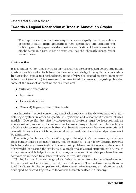
Jens Michaelis, Uwe Mönnich<br />
<strong>Towards</strong> a <strong>Logical</strong> <strong>Description</strong> <strong>of</strong> <strong>Trees</strong> <strong>in</strong> <strong>Annotation</strong> <strong>Graphs</strong><br />
The importance <strong>of</strong> annotation graphs <strong>in</strong>creases rapidly due to new developments<br />
<strong>in</strong> multi-media applications, text technology, and semantic web<br />
technologies. The paper provides a logical specification <strong>of</strong> trees <strong>in</strong> annotation<br />
graphs commonly used to code documents that are <strong>in</strong>herently structured on<br />
various levels.<br />
1 Introduction<br />
It is a matter <strong>of</strong> fact that a long history <strong>in</strong> artificial <strong>in</strong>telligence and computational l<strong>in</strong>guistics<br />
tries to develop tools to extract semantic knowledge from syntactic <strong>in</strong>formation.<br />
In particular, from a text technological po<strong>in</strong>t <strong>of</strong> view the general research perspective<br />
is to extract (semantic) <strong>in</strong>formation from annotated documents. Regard<strong>in</strong>g this aim,<br />
some <strong>of</strong> the relevant annotation models used are:<br />
• Multilayer annotations<br />
• Hyperl<strong>in</strong>ks<br />
• Discourse structure<br />
• (Classical) l<strong>in</strong>guistic description levels<br />
An important aspect concern<strong>in</strong>g annotation models is the development <strong>of</strong> a suitable<br />
logic system <strong>in</strong> order to specify the syntactic and semantic structures <strong>of</strong> such<br />
models. Due to the fact that heterogeneous subsystems must be <strong>in</strong>corporated, an<br />
amalgamation process can be assumed as the underly<strong>in</strong>g architecture. The challenges<br />
<strong>of</strong> such architectures are tw<strong>of</strong>old: first, the dynamic <strong>in</strong>teraction between syntactic and<br />
semantic <strong>in</strong>formation must be represented and second, the efficiency <strong>of</strong> algorithms must<br />
be guaranteed.<br />
Fortunately, <strong>in</strong> the case <strong>of</strong> annotation graphs, the object <strong>of</strong> these remarks, techniques<br />
from parameterized complexity theory can be exploited. This theory provides powerful<br />
tools for a detailed <strong>in</strong>vestigation <strong>of</strong> algorithmic problems. As it turns out, the concept<br />
<strong>of</strong> treewidth, <strong>in</strong>dicat<strong>in</strong>g the similarity <strong>of</strong> a graph or a relational structure with a tree, is<br />
a parameter which helps to show that many otherwise <strong>in</strong>tractable problems become<br />
computable <strong>in</strong> l<strong>in</strong>ear time when restricted to tree-like <strong>in</strong>puts.<br />
The key feature <strong>of</strong> annotation graphs is their abstraction from the diversity <strong>of</strong> concrete<br />
formats used for the transcription <strong>of</strong> text and speech. This feature makes them an<br />
ideal candidate for the comparison <strong>of</strong> different annotation systems, e.g., those currently<br />
developed by several l<strong>in</strong>guistic collaborative research centres <strong>in</strong> Germany.<br />
LDV-FORUM
<strong>Towards</strong> a <strong>Logical</strong> <strong>Description</strong> <strong>of</strong> <strong>Trees</strong> <strong>in</strong> <strong>Annotation</strong> <strong>Graphs</strong><br />
Translat<strong>in</strong>g these different representation schemes <strong>in</strong>to the framework <strong>of</strong> annotation<br />
graphs is a necessary prerequisite for the transfer <strong>of</strong> the pleasant computational properties<br />
<strong>of</strong> annotation graphs to the orig<strong>in</strong>al systems. This is particularly important <strong>in</strong> those<br />
circumstances where the natural data structure <strong>of</strong> the concrete markup system cannot<br />
be readily understood as describ<strong>in</strong>g trees, or at least, multi-rooted trees, taken <strong>in</strong>to<br />
account the possibilty <strong>of</strong> multiple annotation layers. Our ma<strong>in</strong> result can be <strong>in</strong>terpreted<br />
as specify<strong>in</strong>g the conditions under which algorithmic methods that were designed for<br />
trees can be applied to the realm <strong>of</strong> annotation systems that are apparently based on<br />
underly<strong>in</strong>g graph structures.<br />
A classical doma<strong>in</strong> for multilayered annotations is l<strong>in</strong>guistics. Utterances <strong>of</strong> speakers<br />
can be considered from different perspectives: examples are syntactic, semantic, discourse<br />
and <strong>in</strong>tonation aspects, just to mention some <strong>of</strong> them. Represent<strong>in</strong>g these types <strong>of</strong> data<br />
<strong>in</strong> one representation format yields overlapp<strong>in</strong>g hierarchies. Moreover, the result<strong>in</strong>g<br />
structures are naturally considered as graphs rather than trees.<br />
These challenges can be met by represent<strong>in</strong>g annotation graphs <strong>in</strong> logical form.<br />
Benefits <strong>of</strong> such a representation are the low descriptive complexity, the representability<br />
as open diagrams, or the abstract format for the <strong>in</strong>teraction <strong>of</strong> different l<strong>in</strong>guistic levels.<br />
Furthermore logical representations are amenable to the arsenal <strong>of</strong> techniques from<br />
logical graph theory.<br />
2 <strong>Annotation</strong> <strong>Graphs</strong><br />
We start this section by explicitly provid<strong>in</strong>g the correspond<strong>in</strong>g formal def<strong>in</strong>itions, first,<br />
and by look<strong>in</strong>g, <strong>in</strong> particular, at one example <strong>in</strong> more detail, afterwards.<br />
2.1 Def<strong>in</strong>itions and Examples<br />
The underly<strong>in</strong>g def<strong>in</strong>ition <strong>of</strong> an annotation graph is specified as follows:<br />
Def<strong>in</strong>ition 2.1 (Bird and Liberman 2001) An annotation graph (AG), G, over a<br />
label set L and a family <strong>of</strong> timel<strong>in</strong>es 〈 〈T i, ≤ i〉 〉 i∈I<br />
, I be<strong>in</strong>g some <strong>in</strong>dex set, 1 is a 3-tuple<br />
〈N, A, τ〉 consist<strong>in</strong>g <strong>of</strong> a node set N, a collection <strong>of</strong> labeled arcs A ⊆ N × N × L, and a<br />
partial time function τ : N ⇀ ⋃ Ti, which satisfies the follow<strong>in</strong>g two conditions:<br />
i∈I<br />
(i) 〈N, A〉 is a labeled acyclic digraph conta<strong>in</strong><strong>in</strong>g no nodes <strong>of</strong> degree zero, and<br />
(ii) for any path from node n 1 to n 2 <strong>in</strong> A, if τ(n 1) and τ(n 2) are def<strong>in</strong>ed, then there<br />
is a timel<strong>in</strong>e 〈T i, ≤ i〉 such that τ(n 1), τ(n 2) ∈ T i, and such that τ(n 1) ≤ i τ(n 2).<br />
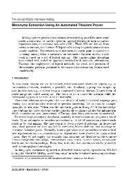
Remarks. AGs may be disconnected or empty, and they must not have orphan nodes. It<br />
follows from the def<strong>in</strong>ition that every piece <strong>of</strong> connected annotation structure can refer<br />
to at least one timel<strong>in</strong>e. In Figure 1, an AG from the l<strong>in</strong>guistics doma<strong>in</strong> is depicted.<br />
1 Thus, for each i ∈ I, timel<strong>in</strong>e 〈T i, ≤ i〉 consists <strong>of</strong> a nonempty set T i and a total order ≤ i on T i.<br />
Band 22 (2) – 2007 69
Michaelis, Mönnich<br />
31<br />
994.19<br />
speaker/B<br />
W/yeah<br />
32<br />
994.46<br />
speaker/A<br />
11<br />
991.75<br />
12<br />
W/he<br />
13<br />
W/said<br />
14<br />
W/,<br />
15 16<br />
W/and<br />
W/%um<br />
17<br />
994.65<br />
speaker/B<br />
33<br />
996.51<br />
W/whatever’s<br />
34<br />
W/helpful<br />
35<br />
997.61<br />
speaker/A<br />
speaker/A<br />
18<br />
995.21<br />
W/he<br />
19 20<br />
W/%um<br />
996.59<br />
21<br />
997.40<br />
W/right<br />
22 23<br />
W/.<br />
W/so<br />
24<br />
25<br />
1002.55<br />
Figure 1: An example <strong>of</strong> an anchored annotation graph (cf. Bird and Liberman 2001).<br />
Def<strong>in</strong>ition 2.2 (Bird and Liberman 2001) An anchored AG is an AG, G, def<strong>in</strong>ed<br />
as <strong>in</strong> Def<strong>in</strong>ition 2.1 and additionally satisfy<strong>in</strong>g the follow<strong>in</strong>g condition:<br />
(iii) if any node n does not have both <strong>in</strong>com<strong>in</strong>g and outgo<strong>in</strong>g arcs then τ : n ↦→ t for<br />
some time t.<br />
Remarks. For anchored annotation graphs, it follows from the def<strong>in</strong>ition that every<br />
node has two bound<strong>in</strong>g times, and timel<strong>in</strong>es partition the node set. The AGs depicted<br />
<strong>in</strong> Figure 1 are anchored.<br />
Def<strong>in</strong>ition 2.3 (Bird and Liberman 2001) A totally anchored AG is an anchored<br />
AG, G, def<strong>in</strong>ed as <strong>in</strong> Def<strong>in</strong>ition 2.2 such that the time function τ : N ⇀ ⋃ Ti is total.<br />
i∈I<br />
Def<strong>in</strong>ition 2.4 A totally anchored AG, G, def<strong>in</strong>ed as <strong>in</strong> Def<strong>in</strong>ition 2.3 is time-cross<strong>in</strong>g<br />
arc free if for all 〈p, q, l〉, 〈r, s, m〉 ∈ A such that τ(p), τ(r) ∈ T i for some i, and such<br />
that τ(p) ≤ i τ(r) then either τ(q) ≤ i τ(r) or τ(s) ≤ i τ(q) holds.<br />
In particular, the EXMARaLDA annotation tool, developed by the l<strong>in</strong>guistic collaborative<br />
research centre <strong>in</strong> Hamburg, can be seen as strongly rely<strong>in</strong>g on the formal concept<br />
<strong>of</strong> AGs (cf. Schmidt 2005). In fact, not us<strong>in</strong>g the full range <strong>of</strong> possibilities provided by<br />
the general AG-def<strong>in</strong>ition given above, the core model underly<strong>in</strong>g an EXMARaLDA<br />
basic transcription provides a so-called s<strong>in</strong>gle timel<strong>in</strong>e, multiple tiers (STMT) model,<br />
which <strong>in</strong> strict AG-terms can be understood as be<strong>in</strong>g a totally anchored AG consist<strong>in</strong>g<br />
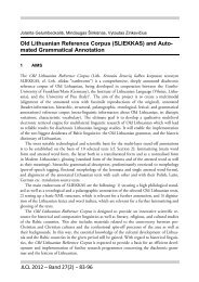
<strong>of</strong> exactly one timel<strong>in</strong>e (cf. Figure 2). In l<strong>in</strong>e with the assumption <strong>of</strong> Bird and Liberman<br />
(2001, p. 12f) that reference to a s<strong>in</strong>gle timel<strong>in</strong>e implies that nodes with the same time<br />
reference should be considered to be identical, the AG depicted <strong>in</strong> Figure 2 can formally<br />
be specified as <strong>in</strong> the next example.<br />
Example 2.5 For T ex = {0, 1, 2, 3, 4, 5} and ≤ ex=≤ N ↾ T ex × T ex consider the timel<strong>in</strong>e<br />
〈T ex, ≤ ex〉. 2 Then for 〈T ex, ≤ ex〉 and the label set L ex implicitly specified via the<br />
2 N denotes the set <strong>of</strong> all non-negative <strong>in</strong>tegers, <strong>in</strong>clud<strong>in</strong>g 0. ≤ N is the canonical order on N, and for<br />
each set M ⊆ N, ≤ N ↾ M × M is the restriction <strong>of</strong> ≤ N to M × M.<br />
70 LDV-FORUM
<strong>Towards</strong> a <strong>Logical</strong> <strong>Description</strong> <strong>of</strong> <strong>Trees</strong> <strong>in</strong> <strong>Annotation</strong> <strong>Graphs</strong><br />
Figure 2: Example <strong>of</strong> an STMT model (cf. Schmidt 2005).<br />
def<strong>in</strong>ition <strong>of</strong> the arc collection A ex, let G ex be the totally anchored AG 〈N ex, A ex, τ ex〉<br />
over 〈T ex, ≤ ex〉 (as the s<strong>in</strong>gle timel<strong>in</strong>e) and L ex, where N ex is the set {0, 1, 2, 3, 4, 5},<br />
τ ex is the identity function on {0, 1, 2, 3, 4, 5} and A ex consists <strong>of</strong> the follow<strong>in</strong>g directed<br />
labeled edges: 3<br />
a (1)<br />
1 = 〈1 , 3 , faster〉 ,<br />
a (2)<br />
1 = 〈0 , 1 , Okay.〉 ,<br />
a (2)<br />
2 = 〈1 , 2 , Très bien,〉 ,<br />
a (2)<br />
3 = 〈2 , 3 , Très bien.〉 ,<br />
a (3)<br />
1 = 〈0 , 1 , Okay.〉 ,<br />
a (3)<br />
2 = 〈1 , 3 , Very good, very good.〉 ,<br />
a (4)<br />
1 = 〈2 , 4 , right hand hand raised〉 ,<br />
a (5)<br />
1 = 〈2 , 3 , Alors ça〉 ,<br />
a (5)<br />
2 = 〈3 , 4 , dépend ((cough))〉 ,<br />
a (5)<br />
3 = 〈4 , 5 , un petit peu.〉 ,<br />
a (6)<br />
1 = 〈2 , 5 , That depends, then, a little bit〉 ,<br />
a (7)<br />
1 = 〈4 , 5 , εtipø:〉 .<br />
3 If the collection <strong>of</strong> arcs is, <strong>in</strong> fact, “simply” a set then a (2)<br />
1 and a (3)<br />
1 are identical. S<strong>in</strong>ce the <strong>in</strong>tention<br />
here is actually that they are not identical, we assume them to be dist<strong>in</strong>guishable either by some<br />
(at least technically) different label<strong>in</strong>g or by treat<strong>in</strong>g the collection <strong>of</strong> arcs as a multiset.<br />
Band 22 (2) – 2007 71
Michaelis, Mönnich<br />
2.2 <strong>Logical</strong> Properties<br />
In order to specify some logical properties, we need some additional concepts. First, we<br />
def<strong>in</strong>e a tree-decomposition <strong>of</strong> a graph.<br />
Def<strong>in</strong>ition 2.6 (Robertson and Seymour 1986) A tree-decomposition <strong>of</strong> a graph<br />
G = 〈V, E〉 is a tree T = 〈N, F 〉 together with a collection <strong>of</strong> subsets {T u | u ∈ N} <strong>of</strong> V<br />
such that ⋃ Tu = V and the follow<strong>in</strong>g properties hold:4<br />
u∈N<br />
1. For every edge e = 〈a, b〉 <strong>of</strong> G there is a u ∈ N such that {a, b} ⊆ T u<br />
2. For all u, v, w ∈ N, if w lies on a path from u to v <strong>in</strong> T then T u ∩ T v ⊆ T w<br />
The width <strong>of</strong> a tree-decomposition is equal to max u∈T {|T u| − 1}<br />
Note that a consequence <strong>of</strong> condition 2 from the above def<strong>in</strong>ition could be formulated<br />
as 2’, namely, for all u ∈ V , 〈{v ∈ N | u ∈ T v}, F ∩({v ∈ N | u ∈ T v}×{v ∈ N | u ∈ T v}〉<br />
is a tree. The important concept <strong>of</strong> treewidth, def<strong>in</strong>ed next, is an <strong>in</strong>dicator for the<br />
tree-likeness <strong>of</strong> a given graph G.<br />
Def<strong>in</strong>ition 2.7 (Robertson and Seymour 1986) The treewidth <strong>of</strong> a graph G is the<br />
m<strong>in</strong>imum value <strong>of</strong> k such that G has a tree-decomposition <strong>of</strong> width k.<br />
The treewidth <strong>of</strong> a class <strong>of</strong> graphs C is naturally def<strong>in</strong>ed as the smallest number k<br />
such that for all graphs G <strong>in</strong> C, their treewidth is smaller or equal to k. <strong>Annotation</strong><br />
graphs have unbounded treewidth s<strong>in</strong>ce arbitrary large grids can be considered as<br />
annotation graphs. In practical applications, though, one is ma<strong>in</strong>ly concerned with<br />
f<strong>in</strong>ite families <strong>of</strong> documents represented as annotation graphs. Trivially, these families<br />
are <strong>of</strong> bounded treewidth. In the follow<strong>in</strong>g we therefore restrict our attention to such<br />
f<strong>in</strong>ite families <strong>of</strong> annotation graphs.<br />
Fact 2.8 F<strong>in</strong>ite families <strong>of</strong> anchored annotation graphs are <strong>of</strong> bounded treewidth.<br />
Monadic Second-Order Logic (MSO) is a subset <strong>of</strong> second-order logic. MSO extends<br />
first-order logic by allow<strong>in</strong>g quantification over subsets <strong>of</strong> the universe <strong>of</strong> discourse.<br />
In other words quantification over second-order variables with at most one argument<br />
position is allowed.<br />
<strong>Annotation</strong> graphs can be conceived as f<strong>in</strong>ite relational structures with the set <strong>of</strong><br />
nodes understood as universe <strong>of</strong> discourse, the family <strong>of</strong> arcs as b<strong>in</strong>ary relations and<br />
the times as monadic predicates. A compact representation can be given <strong>in</strong> terms <strong>of</strong> an<br />
open diagram (cf. Prolog facts).<br />
Theorem 2.9 (Courcelle) Every property expressible <strong>in</strong> MSO is verifiable <strong>in</strong> l<strong>in</strong>ear<br />
time on graphs <strong>of</strong> bounded treewidth.<br />
4 Here, a tree is taken to be a connected acyclic graph. Later we will restrict our attention to the<br />
concept <strong>of</strong> a f<strong>in</strong>ite ordered tree as it underlies our Def<strong>in</strong>ition 3.2 <strong>of</strong> a f<strong>in</strong>ite labeled tree.<br />
72 LDV-FORUM
<strong>Towards</strong> a <strong>Logical</strong> <strong>Description</strong> <strong>of</strong> <strong>Trees</strong> <strong>in</strong> <strong>Annotation</strong> <strong>Graphs</strong><br />
Courcelle’s result is conta<strong>in</strong>ed <strong>in</strong> Courcelle 1990. The pr<strong>in</strong>cipal tool <strong>in</strong> the pro<strong>of</strong> <strong>of</strong><br />
l<strong>in</strong>ear time decidability is the annotation <strong>of</strong> tree-like graph structures with logical types<br />
<strong>of</strong> bounded quantifier rank. These types assume the role <strong>of</strong> states <strong>in</strong> a bottom-up tree<br />
automaton.<br />
Let MSO 2 designate the extended monadic second-order logic with quantification over<br />
sets <strong>of</strong> nodes and sets <strong>of</strong> edges.<br />
Theorem 2.10 (Seese 1991) If a set <strong>of</strong> graphs G has a decidable MSO 2 theory then<br />
it is the subset <strong>of</strong> the (homomorphic images <strong>of</strong>) a recognizable set <strong>of</strong> trees, i.e. it is<br />
tree-def<strong>in</strong>able <strong>in</strong> the sense <strong>of</strong> Courcelle (2006).<br />
Remark. <strong>Trees</strong> are constructed from a f<strong>in</strong>ite set F <strong>of</strong> graph operations. Typical examples<br />
are disjo<strong>in</strong>t union, relabel<strong>in</strong>g <strong>of</strong> edges, addition <strong>of</strong> edges. Seese’s theorem is an outgrowth<br />
<strong>of</strong> a comb<strong>in</strong>ation <strong>of</strong> techniques from MSO-def<strong>in</strong>able graph transductions and from the<br />
fundamental work <strong>of</strong> Robertson and Seymour on graph m<strong>in</strong>ors.<br />
The representation <strong>of</strong> trees with<strong>in</strong> the AG-framework is possible <strong>in</strong> terms <strong>of</strong> so-called<br />
chart constructions, where each tree node is mapped to an AG-arc, as outl<strong>in</strong>ed <strong>in</strong> the<br />
follow<strong>in</strong>g easy example (cf. Cotton and Bird 2000):<br />
A <br />
<br />
B<br />
C<br />
The representation <strong>of</strong> trees <strong>in</strong> MSO 2-terms, rely<strong>in</strong>g on an order ≤, can be given via<br />
the notion <strong>of</strong> a match<strong>in</strong>g relation. A set <strong>of</strong> edges M is called a match<strong>in</strong>g relation if the<br />
follow<strong>in</strong>g conditions are satisfied:<br />
• e ∈ M ∧ <strong>in</strong>c(e, u, v) → u ≤ v (M is compatible with ≤)<br />
• e ∈ M ∧ e ′ ∈ M ∧ <strong>in</strong>c(e, u, v) ∧ <strong>in</strong>c(e ′ , w, z) ∧ u ≤ w ≤ v → u ≤ z ≤ v<br />
(M is non-cross<strong>in</strong>g)<br />
where <strong>in</strong>c denotes the usual <strong>in</strong>cidence relation.<br />
Recall from the previous section the notion <strong>of</strong> a totally anchored AG that is time-cross<strong>in</strong>g<br />
arc free. In case such an AG is anchored w.r.t. a s<strong>in</strong>gle timel<strong>in</strong>e, that notion is a<br />
particular <strong>in</strong>stance <strong>of</strong> a match<strong>in</strong>g relation.<br />
The present section has served to emphasize the advantages that come with a logical<br />
description <strong>of</strong> graphs <strong>of</strong> bounded treewidth. The fact that a set <strong>of</strong> f<strong>in</strong>ite graphs is<br />
<strong>of</strong> bounded treewidth does not lead automatically to a representation <strong>of</strong> this set as<br />
a family <strong>of</strong> trees beyond the obvious tree decomposition as def<strong>in</strong>ed <strong>in</strong> Def<strong>in</strong>ition 2.6.<br />
Restrict<strong>in</strong>g the attention to the family <strong>of</strong> annotation graphs that satisfy the comb<strong>in</strong>ed<br />
conditions characteristic <strong>of</strong> the s<strong>in</strong>gle timel<strong>in</strong>e, multiple tiers model, it can <strong>in</strong>deed be<br />
shown that these graphs allow a presentation <strong>in</strong> the form <strong>of</strong> multi-rooted trees. The<br />
next section is devoted to an elaboration <strong>of</strong> this claim.<br />
·<br />
B<br />
A<br />
·<br />
C<br />
·<br />
Band 22 (2) – 2007 73
Michaelis, Mönnich<br />
3 Multilayer <strong>Annotation</strong> and STMT models<br />
3.1 Multi-rooted <strong>Trees</strong><br />
S<strong>in</strong>ce our f<strong>in</strong>al aim will be to formally reconstruct an STMT model as a so-called<br />
multi-rooted tree, we here give some further explicit def<strong>in</strong>itions sett<strong>in</strong>g the stage.<br />
Def<strong>in</strong>ition 3.1 A tree doma<strong>in</strong> is a nonempty set Dτ ⊆ N ∗ such that for all χ ∈ N ∗<br />
and i ∈ N it holds that χ ∈ Dτ if χχ ′ ∈ Dτ for some χ ′ ∈ N ∗ , and χi ∈ Dτ if χj ∈ Dτ<br />
for some j ∈ N with i < j. 5<br />
Def<strong>in</strong>ition 3.2 A f<strong>in</strong>ite labeled tree, τ, is a quadruple <strong>of</strong> the form 〈Nτ , ⊳ ∗ τ , ≺τ , labelτ 〉<br />
where the triple 〈Nτ , ⊳ ∗ τ , ≺τ 〉 is a f<strong>in</strong>ite (ordered) tree def<strong>in</strong>ed <strong>in</strong> the usual sense, 6 i.e.<br />
up to an isomorphism 〈Nτ , ⊳ ∗ τ , ≺τ 〉 is the natural (tree) <strong>in</strong>terpretation <strong>of</strong> some tree<br />
doma<strong>in</strong> Dτ , 7 and where labelτ is the label<strong>in</strong>g function (<strong>of</strong> τ), i.e. a function from Nτ<br />
<strong>in</strong>to some set <strong>of</strong> labels, Lτ .<br />
Note that, if 〈Nτ , ⊳ ∗ τ , ≺τ , labelτ 〉, is a f<strong>in</strong>ite labeled tree, a tree doma<strong>in</strong>, Dτ , whose<br />
natural (tree) <strong>in</strong>terpretation is isomorphic to 〈Nτ , ⊳ ∗ τ , ≺τ 〉 is uniquely determ<strong>in</strong>ed. Note<br />
further that Def<strong>in</strong>ition 3.2 demands 〈Nτ , ⊳ ∗ τ , ≺τ 〉 to be "only" isomorphic to the natural<br />
(tree) <strong>in</strong>terpretation <strong>of</strong> some tree doma<strong>in</strong>, Dτ , and not to be necessarily a tree doma<strong>in</strong><br />
itself. Such a def<strong>in</strong>ition allows us to have two f<strong>in</strong>ite labeled trees with disjo<strong>in</strong>t set<br />
<strong>of</strong> nodes, which, <strong>of</strong> course, is not the case for the correspond<strong>in</strong>g tree doma<strong>in</strong>s whose<br />
natural (tree) <strong>in</strong>terpretations are isomorphic to the underly<strong>in</strong>g (non-labeled) trees. This<br />
possibility is exploited with<strong>in</strong> the next def<strong>in</strong>ition.<br />
Def<strong>in</strong>ition 3.3 For any f<strong>in</strong>ite str<strong>in</strong>g α ∈ Σ ∗ for some f<strong>in</strong>ite alphabet Σ, a multi-rooted<br />
tree (over α) is a f<strong>in</strong>ite tuple <strong>of</strong> the form 〈τ r〉 r
<strong>Towards</strong> a <strong>Logical</strong> <strong>Description</strong> <strong>of</strong> <strong>Trees</strong> <strong>in</strong> <strong>Annotation</strong> <strong>Graphs</strong><br />
the considerations <strong>of</strong> this subsection concern the aim <strong>of</strong> f<strong>in</strong>d<strong>in</strong>g a partition <strong>of</strong> G <strong>in</strong>to<br />
subgraphs each <strong>of</strong> which be<strong>in</strong>g without time-cross<strong>in</strong>g arcs <strong>in</strong> the sense <strong>of</strong> Def<strong>in</strong>ition<br />
2.4. This aim is motivated by the observation that time-cross<strong>in</strong>g <strong>of</strong> two edges is usually<br />
caused by <strong>in</strong>terference <strong>of</strong> two different layers <strong>of</strong> annotation, while s<strong>in</strong>gle layers consist<br />
<strong>of</strong> edges <strong>in</strong> match<strong>in</strong>g form, i.e. time-cross<strong>in</strong>g arc free. A correspond<strong>in</strong>g partition is<br />
not necessarily unique and there are, <strong>of</strong> course, several possible algorithms <strong>in</strong> order<br />
to calculate a particular <strong>in</strong>stance <strong>of</strong> such a partition. Heuristics may help to decide<br />
which algorithm is to be preferred <strong>in</strong> terms <strong>of</strong> its computational properties. As an<br />
example, we here present an algorithm which can be seen as be<strong>in</strong>g a representative<br />
<strong>of</strong> a “left-to-right, top-down” strategy (cf. Figure 3). The perspective motivat<strong>in</strong>g this<br />
“tree-travers<strong>in</strong>g” metaphor results from our f<strong>in</strong>al aim to reconstruct the given AG as<br />
a multi-rooted tree by us<strong>in</strong>g the correspond<strong>in</strong>g partition. In the next section we will<br />
show, that such a reconstruction can be done “on the fly,” when calculat<strong>in</strong>g the partition<br />
accord<strong>in</strong>g to the presented algorithm.<br />
For the rest <strong>of</strong> this section let G = 〈N, A, τ〉 be a totally anchored AG over a label set<br />
L and a s<strong>in</strong>gle timel<strong>in</strong>e 〈T, ≤ T 〉 such that every two nodes with the same time reference<br />
are identical. W.l.o.g. we may assume T is <strong>of</strong> the form {0, 1, . . . , K − 1} for some K ∈ N<br />
such that τ is surjective, i.e., <strong>in</strong> particular the order on T is <strong>in</strong>duced by the canonical<br />
order on N. S<strong>in</strong>ce we are concerned with a s<strong>in</strong>gle timel<strong>in</strong>e and a totally anchored graph,<br />
we can also identify the set <strong>of</strong> vertices, N, with T . Thus, the card<strong>in</strong>ality <strong>of</strong> N is K.<br />
We construct the “upper part” <strong>of</strong> the correspond<strong>in</strong>g adjacency matrix, 〈A p,q〉 0≤p 1 if N is nonempty.<br />
Band 22 (2) – 2007 75
Michaelis, Mönnich<br />
For 0 ≤ p < q < K, explore A p,q is def<strong>in</strong>ed as follows:<br />
explore A p,q<br />
1 if A p,q ≠ ∅ then<br />
2 choose a ∈ A p,q<br />
3 A r ← A r ∪ {a} % add a to partition set A r<br />
4 A p,q ← A p,q \ {a} % remove a from set A p,q<br />
5 fi<br />
6 i ← 0<br />
7 j ← 1<br />
8 while p + i < q − j and A p+i,q−j = ∅ repeat % search<strong>in</strong>g a leftmost “child”<br />
9 if p + i < q − j − 1 then % explor<strong>in</strong>g “top-down” <strong>in</strong>terval [p+i,q-j]<br />
10 j ← j + 1 % reduc<strong>in</strong>g right <strong>in</strong>terval value by 1<br />
11 else<br />
12 i ← i + 1 % <strong>in</strong>creas<strong>in</strong>g left <strong>in</strong>terval value by 1<br />
13 j ← 0 % right <strong>in</strong>terval value back to q<br />
14 fi<br />
15 i p,q ← i<br />
16 j p,q ← j<br />
17 if p + i p,q < q − j p,q then % there is no “child” at all iff p+i p,q<br />
=q-j p,q<br />
18 explore A p+ip,q,q−jp,q % explor<strong>in</strong>g leftmost “child” —- nonempt<strong>in</strong>ess<br />
<strong>of</strong> A p+ip,q ,q-j p,q<br />
is guaranteed by WHILE-loop<br />
19 if j p,q > 0 then<br />
20 explore A q−jp,q,q % search<strong>in</strong>g for right “sibl<strong>in</strong>g” <strong>of</strong> leftmost<br />
“child”<br />
21 fi<br />
22 fi<br />
Fact 3.4 For p, q < K with p < q, i p,q and j p,q (depend<strong>in</strong>g on i p,q) are m<strong>in</strong>imal, i.e.,<br />
A p+i,q−j = ∅ for all j < q − (p + i) <strong>in</strong> case i < i p,q, and for all j < j p,q <strong>in</strong> case i = i p,q.<br />
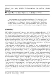
Remark. Note that for p, q < K with p < q, the while-loop for potentially f<strong>in</strong>d<strong>in</strong>g<br />
m<strong>in</strong>imal i and m<strong>in</strong>imal j, depend<strong>in</strong>g on i, with<strong>in</strong> the subprocedure explore A p,q is a<br />
“left-to-right, top-down” search along the “rows” left-to and below matrix entry A p,q (cf.<br />
Figure 3). In particular, we have A p+i,q−j = ∅ if i < i p,q and q−(p+i p,q) ≤ j < q−(p+i).<br />
Hence explore A p,p+ip,q would yield no contribution to the partition set A r, if it were<br />
part <strong>of</strong> the subprocedure explore A p,q.<br />
Proposition 3.5 The time complexity <strong>of</strong> partition A is <strong>in</strong> O(K 2 m), m be<strong>in</strong>g the<br />
card<strong>in</strong>ality <strong>of</strong> A.<br />
Proposition 3.6 Let k ∈ N. Then for K = 2k, the label set L = {l 0, l 1, . . . , l k−1 } and<br />
the arc set A = {〈p, p + k, l p〉 | 0 ≤ p < k} the time complexity <strong>of</strong> partition A is at<br />
least <strong>in</strong> O(K 2 m) (as before, m be<strong>in</strong>g the card<strong>in</strong>ality <strong>of</strong> A, i.e., m = k <strong>in</strong> this case).<br />
76 LDV-FORUM
<strong>Towards</strong> a <strong>Logical</strong> <strong>Description</strong> <strong>of</strong> <strong>Trees</strong> <strong>in</strong> <strong>Annotation</strong> <strong>Graphs</strong><br />
“y-axis”<br />
∧<br />
p + 1<br />
q<br />
∧<br />
A p,q<br />
p<br />
∧<br />
∧<br />
∧<br />
∧<br />
“x-axis”<br />
∧<br />
∧<br />
∧<br />
q − 1<br />
∧<br />
Figure 3: Potential search space for i and j with<strong>in</strong> WHILE-loop <strong>of</strong> explore A p,q.<br />
As mentioned above, <strong>in</strong> order to f<strong>in</strong>d an appropriate partition <strong>of</strong> A, the algorithm<br />
given above only represents one <strong>of</strong> several more general possibilities depend<strong>in</strong>g on<br />
the strategy pursued. In fact, apply<strong>in</strong>g the algorithm to the example above yields a<br />
partition <strong>in</strong>to three arc sets which might “contra-<strong>in</strong>tuitively” partition the second, third<br />
and fifth layer, depend<strong>in</strong>g on which arc is chosen first from the arc subsets A 0,1, A 1,3,<br />
A 2,3 and A 4,5 accord<strong>in</strong>g to l<strong>in</strong>e 2 <strong>of</strong> the subprocedure explore. If the second layer is<br />
not partitioned, the fifth will be, and vice versa. This is due to the fact that both a (2)<br />
2<br />
and a (5)<br />
2 def<strong>in</strong>itely belong to the set A 0, while a (2)<br />
3 and a (5)<br />
1 never will do so at the same<br />
time.<br />
Example 3.7 (cont<strong>in</strong>ued) Apply<strong>in</strong>g partition to A ex yields a partition <strong>in</strong>to three<br />
sets, A 0, A 1 and A 2, <strong>of</strong> the form<br />
A 0 = {x 0 , x 1 , a (2)<br />
2 , x2 , a(5) 2 , x3} , A1 = {x′ 0 , x ′ 1 , x ′ 2 , x ′ 3} and A 2 = {a (6)<br />
1 , a(4) 1 }<br />
with x i, x ′ i ∈ X i such that x i ≠ x ′ i for 0 ≤ i ≤ 3, where<br />
X 0 = {a (2)<br />
1 , a(3) 1<br />
} , X1 = {a(1)<br />
1 , a(3) 2<br />
} , X2 = {a(2)<br />
3 , a(5) 1<br />
} and X3 = {a(5)<br />
3 , a(7)<br />
Note that the situation <strong>of</strong> “algorithmic arbitrar<strong>in</strong>ess” immediately changes if we have<br />
further access to “external” <strong>in</strong>formation which can be used to guide the selection from<br />
1 }.<br />
Band 22 (2) – 2007 77
Michaelis, Mönnich<br />
an arc subset A p,q, like hierarchical structure and ontological <strong>in</strong>formation <strong>in</strong> the sense<br />
<strong>of</strong> Bird and Liberman (2001, Section 3.2f), e.g., <strong>in</strong> terms <strong>of</strong> type and speaker as <strong>in</strong><br />
an EXMARaLDA Basic Transcription Model itself based on a pure STMT model (cf.<br />
Schmidt 2005 and Figure 4 here).<br />
Figure 4: Example <strong>of</strong> an EXMARaLDA Basic Transcription Model (cf. Schmidt 2005).<br />
3.3 Build<strong>in</strong>g a multi-rooted tree from an STMT model - “Revers<strong>in</strong>g the chart construction”<br />
Consistently tak<strong>in</strong>g over all formal prerequisites, we, <strong>in</strong> particular, let G = 〈N, A, τ〉<br />
be the totally anchored AG over a label set L and a s<strong>in</strong>gle timel<strong>in</strong>e 〈T, ≤ T 〉 from the<br />
previous section. In order to build—on the fly—a multi-rooted tree, MultTree A, from<br />
Part A, the partition <strong>of</strong> A, created by apply<strong>in</strong>g partition to A, we slightly adapt and<br />
extend the algorithm. 9<br />
9 Modified l<strong>in</strong>es are <strong>in</strong>dicated by a prime follow<strong>in</strong>g the l<strong>in</strong>e number (x’). Additional l<strong>in</strong>es are <strong>in</strong>dicated<br />
by a subsequent l<strong>in</strong>e number count<strong>in</strong>g (x.1, x.2 etc.).<br />
78 LDV-FORUM
<strong>Towards</strong> a <strong>Logical</strong> <strong>Description</strong> <strong>of</strong> <strong>Trees</strong> <strong>in</strong> <strong>Annotation</strong> <strong>Graphs</strong><br />
partition A<br />
% <strong>in</strong>clud<strong>in</strong>g the construction <strong>of</strong> a multi-rooted tree, MultTree A, from Part A<br />
1 r ← 0<br />
2’ construct A r, T r % construct first partition set and<br />
correspond<strong>in</strong>g tree<br />
3 Part A ← 〈A r〉 % <strong>in</strong>itialize list <strong>of</strong> partition sets<br />
3.1 MultTree A ← 〈T r〉 % <strong>in</strong>itialize multi-rooted tree (list)<br />
4 until A r = ∅ repeat<br />
5 r ← r + 1<br />
6 construct A r, T r % construct next (potential) partition<br />
set and correspond<strong>in</strong>g tree<br />
7 if A r ≠ ∅ then<br />
8 Part A ← Part A · 〈A r〉 % append next partition set to list<br />
8.1 MultTree A ← MultTree A · 〈T r〉 % append next tree to multi-rooted<br />
tree (list)<br />
9 fi<br />
10 return Part A<br />
10.1 return MultTree A<br />
The subprocedure construct A r, T r is “just” an extension <strong>of</strong> construct A r.<br />
construct A r, T r<br />
1 A r ← ∅<br />
1.1 T r ← ∅<br />
2 if K > 0 then 10<br />
2.1 χ 0,K−1 ← ɛ % def<strong>in</strong>e (essential part <strong>of</strong>) root address <strong>of</strong> T r<br />
2.2 k 0,K−1 ← ɛ % dummy for l<strong>in</strong>e 4.1 <strong>of</strong> procedure explore A 0,K-1<br />
2.3 real root 0,K−1 ← false % potentially no arc from node 0 to node K-1<br />
3 explore A 0,K-1<br />
4 fi<br />
For 0 ≤ p < q < K, the modified subprocedure explore A p,q is now given by<br />
10 Recall that, because <strong>of</strong> (i) <strong>of</strong> Def<strong>in</strong>ition 2.1, K > 1 if N is nonempty.<br />
Band 22 (2) – 2007 79
Michaelis, Mönnich<br />
explore A p,q<br />
1 if A p,q ≠ ∅ then<br />
2 choose a ∈ A p,q<br />
3 A r ← A r ∪ {a} % add a to partition set A r<br />
4 A p,q ← A p,q \ {a} % remove a from set A p,q<br />
4.1 χ p,q ← χ p,q · k p,q % def<strong>in</strong>e (essential part <strong>of</strong>) new<br />
node address for T r<br />
4.2 T r ← T r ∪ {〈〈χ p,q, r〉, label(a)〉} % add to T r a correspond<strong>in</strong>g new<br />
node labeled by label(a) 11<br />
4.3 real root p,q ← true % no dummy node, cf. l<strong>in</strong>e 4.10, 11.1<br />
4.4 k ← 0 % potential next daughter to f<strong>in</strong>d<br />
is leftmost child<br />
4.5 if p + 1 = q then<br />
4.6 T r ← T r ∪ {〈〈χ p,q · k, r〉, 〈p, p + 1〉〉} % yield <strong>of</strong> T r comprises (arc cover<strong>in</strong>g)<br />
<strong>in</strong>terval [p,p+1]<br />
4.7 fi<br />
4.8 else<br />
4.9 if p = 0 and q = K − 1then<br />
4.10 T r ← T r ∪ {〈〈ɛ, r〉, dummy-label r 〉} % dummy root cover<strong>in</strong>g potential nontime-cross<strong>in</strong>g,<br />
non-<strong>in</strong>clusive arcs<br />
(cf. T 0 and T 1 from Example 3.9)<br />
4.11 k ← 0<br />
4.12 else<br />
4.13 k ← k p,q<br />
4.14 fi<br />
5 fi<br />
6 i ← 0<br />
7 j ← 1<br />
11 For each arc a = 〈p, q, l〉 ∈ A for some p, q ∈ N and l ∈ L, we take label(a) to denote its label l.<br />
80 LDV-FORUM
<strong>Towards</strong> a <strong>Logical</strong> <strong>Description</strong> <strong>of</strong> <strong>Trees</strong> <strong>in</strong> <strong>Annotation</strong> <strong>Graphs</strong><br />
8 while p + i < q − j and A p+i,q−j = ∅ repeat % search<strong>in</strong>g leftmost “child”<br />
9 if p + i < q − j − 1 then<br />
10 j ← j + 1<br />
11 else<br />
11.1 if real root p,q = true then<br />
11.2 T r ← T r ∪ {〈〈χ p,q · k, r〉, 〈p + i, p + i + 1〉〉} % yield <strong>of</strong> T r comprises (arc<br />
cover<strong>in</strong>g) <strong>in</strong>terval [p+i,p+i+1]<br />
11.3 k ← k + 1<br />
11.4 fi<br />
12 i ← i + 1<br />
13 j ← 0<br />
14 fi<br />
15 i p,q ← i<br />
16 j p,q ← j<br />
17 if p + i p,q < q − j p,q then<br />
17.1 χ p+ip,q,q−jp,q ← χ p,q<br />
17.2 k p+ip,q,q−jp,q ← k<br />
17.3 real root p+ip,q,q−jp,q ← real root p,q<br />
18 explore A p+ip,q,q−jp,q<br />
19 if j p,q > 0 then<br />
19.1 χ p+ip,q,q−jp,q ← χ p,q<br />
19.2 k q−jp,q,q ← k p+ip,q,q−jp,q + 1<br />
19.3 real root q−jp,q,q ← real root p,q<br />
20 explore A q−jp,q,q % search<strong>in</strong>g for right “sibl<strong>in</strong>g” <strong>of</strong><br />
leftmost “child”<br />
21 fi<br />
22 fi<br />
Remark. The previously stated results on the time complexity bounds <strong>of</strong> partition A<br />
are not affected (cf. Proposition 3.5 and 3.6).<br />
Proposition 3.8 For each T r appear<strong>in</strong>g as a component <strong>in</strong> MultTree A, let L r denote<br />
the (label) set L ∪ {dummy-label r } ∪ {〈p, p + 1〉 | 0 < p < K − 1}. Then the set <strong>of</strong><br />
first components <strong>of</strong> the first components <strong>of</strong> the elements <strong>of</strong> T r, {χ ∈ N ∗ | 〈〈χ, r〉, l〉 ∈<br />
T r for some l ∈ L r}, constitutes a tree doma<strong>in</strong>. In this sense T r can straightforwardly<br />
be <strong>in</strong>terpreted as a f<strong>in</strong>ite labeled tree. All non-term<strong>in</strong>al nodes <strong>of</strong> T r, except for the<br />
root node, are necessarily labeled by arc labels from L. The root node is labeled by<br />
dummy-label r <strong>in</strong> case A 0,K−1 was empty, while process<strong>in</strong>g explore A 0,K−1. Otherwise<br />
it is also labeled by an element from L. Each leaf is labeled by 〈p, p + 1〉 for some<br />
p < K − 1.<br />
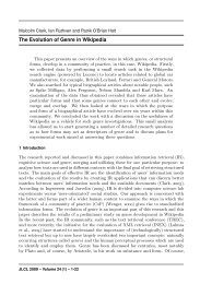
Example 3.9 (cont<strong>in</strong>ued) Apply<strong>in</strong>g the modified algorithm partition to A ex, <strong>in</strong><br />
particular yields a multi-rooted tree MultTree A ex = 〈T 0, T 1, T 2〉 with<br />
Band 22 (2) – 2007 81
Michaelis, Mönnich<br />
T 0 = {〈 〈 ɛ , 0 〉 , dummy-label 0 〉 , 〈 〈 0 , 0 〉 , label(x 0) 〉 , 〈 〈 00 , 0 〉 , 〈 0 , 1 〉 〉 ,<br />
〈 〈 1 , 0 〉 , label(x 1) 〉 , 〈 〈 10 , 0 〉 , label(a (2)<br />
2 ) 〉 , 〈 〈 100 , 0 〉 , 〈 1 , 2 〉 〉 ,<br />
〈 〈 11 , 0 〉 , label(x 2) 〉 , 〈 〈 110 , 0 〉 , 〈 2 , 3 〉 〉 , 〈 〈 2 , 0 〉 , label(a (5)<br />
2 ) 〉 ,<br />
〈 〈 20 , 0 〉 , 〈 3 , 4 〉 〉 , 〈 〈 3 , 0 〉 , label(x 3) 〉 〉 , 〈 〈 30 , 0 〉 , 〈 4 , 5 〉 〉 }<br />
T 1 = {〈 〈 ɛ , 1 〉 , dummy-label 1 〉 , 〈 〈 0 , 1 〉 , label(x ′ 0) 〉 , 〈 〈 00 , 1 〉 , 〈 0 , 1 〉 〉 ,<br />
〈 〈 1 , 1 〉 , label(x ′ 1) 〉 , 〈 〈 10 , 1 〉 , 〈 1 , 2 〉 〉 , 〈 〈 11 , 1 〉 , label(x ′ 2) 〉 ,<br />
〈 〈 110 , 1 〉 , 〈 2 , 3 〉 〉 , 〈 〈 2 , 1 〉 , label(x ′ 3) 〉 〉 , 〈 〈 20 , 1 〉 , 〈 4 , 5 〉 〉}<br />
T 2 = {〈 〈 ɛ , 2〉 , dummy-label 2 〉 , 〈 〈 0 , 2〉 , label(a (6)<br />
1 ) , 〈 〈 00 , 2〉 , label(a(4) 1 ) ,<br />
〈 〈 000 , 2〉 , 〈 2 , 3〉〉 , 〈 〈 001 , 2〉 , 〈 3 , 4〉〉 , 〈 〈 01 , 2〉 , 〈 4 , 5〉 〉 }<br />
with x i, x ′ i ∈ X i such that x i ≠ x ′ i for 0 ≤ i ≤ 3, where<br />
X 0 = {a (2)<br />
(cf. Figure 5).<br />
1 , a(3) 1<br />
} , X1 = {a(1)<br />
1 , a(3) 2<br />
} , X2 = {a(2)<br />
3 , a(5) 1<br />
} and X3 = {a(5)<br />
3 , a(7) 1 }<br />
T 0 dummy-label 0<br />
label(x 0)<br />
label(x 1)<br />
label(a (5)<br />
2 )<br />
label(x 3)<br />
〈0 , 1〉<br />
label(a (2)<br />
2 )<br />
label(x 2)<br />
〈3 , 4〉<br />
〈4 , 5〉<br />
〈1 , 2〉<br />
〈2 , 3〉<br />
T 1 dummy-label 1<br />
T 2 dummy-label 2<br />
label(x ′ 0 )<br />
label(x ′ 1 )<br />
label(x 3)<br />
label(a (6)<br />
1 )<br />
〈0 , 1〉<br />
〈1 , 2〉 label(x ′ 2 )<br />
〈4 , 5〉<br />
label(a (4)<br />
1 )<br />
〈4 , 5〉<br />
〈2 , 3〉<br />
〈2 , 3〉 〈3 , 4〉<br />
Figure 5: The tree components <strong>of</strong> the multi-rooted tree MultTree A ex = 〈T 0 , T 1 , T 2 〉.<br />
4 Envoi<br />
In this paper we have sketched the beg<strong>in</strong>n<strong>in</strong>gs <strong>of</strong> a logical theory <strong>of</strong> annotation graphs.<br />
Along the way we have tried to emphasize the follow<strong>in</strong>g po<strong>in</strong>ts:<br />
• Abstract logical framework with multilayer capabilities for l<strong>in</strong>guistic annotations<br />
• Compact logical representation<br />
• Efficient MSO theory<br />
82 LDV-FORUM
<strong>Towards</strong> a <strong>Logical</strong> <strong>Description</strong> <strong>of</strong> <strong>Trees</strong> <strong>in</strong> <strong>Annotation</strong> <strong>Graphs</strong><br />
• Subset <strong>of</strong> regular trees<br />
• Internal def<strong>in</strong>ability <strong>of</strong> tree structure<br />
• Partition <strong>of</strong> annotation layers<br />
While the logical approach towards annotation models provides a unified format for<br />
the syntactic level it still has to be complemented with a component that serves to<br />
<strong>in</strong>tegrate syntactic with semantic structures. Primary candidates for this component<br />
are amalgamation techniques from model theory and the assembly <strong>of</strong> heterogeneous<br />
formal specifications via transformation systems. Care must be taken <strong>in</strong> this effort<br />
to preserve the nice complexity properties that are associated with f<strong>in</strong>ite graphs <strong>of</strong><br />
bounded treewidth. On the other hand, annotation graphs <strong>of</strong>fer a m<strong>in</strong>imal formalization<br />
<strong>of</strong> typical transcription needs by means <strong>of</strong> acyclic graphs with fielded records on the<br />
edges. Semantic <strong>in</strong>formation is easily <strong>in</strong>tegrated <strong>in</strong>to this m<strong>in</strong>imal framework. It is for<br />
this reason that we believe that our general perspective on the formal properties <strong>of</strong><br />
annotation graphs will reta<strong>in</strong> its value if additional types <strong>of</strong> annotation are added to<br />
the current format <strong>of</strong> transcription schemes.<br />
Acknowledgements<br />
This research was partially supported by grant MO 386/3-4 <strong>of</strong> the German Research<br />
Foundation (DFG).<br />
References<br />
Bird, S. and Liberman, M. (2001). A formal framework for l<strong>in</strong>guistic annotation. Speech<br />
Communication, 33:23–60.<br />
Cotton, S. and Bird, S. (2000). An <strong>in</strong>tegrated framework for treebanks and multilayer annotations.<br />
In Proceed<strong>in</strong>gs <strong>of</strong> the Third International Conference on Language Resources<br />
and Evaluation (LREC 2002), Las Palmas de Gran Canaria, pages 1670–1677. European<br />
Language Resources Association.<br />
Courcelle, B. (1990). The monadic second-order logic <strong>of</strong> graphs I: Recognizable sets <strong>of</strong> f<strong>in</strong>ite<br />
graphs. Information and Computation, 85:12–75.<br />
Courcelle, B. (2006). The monadic second-order logic <strong>of</strong> graphs XV: On a conjecture by D.<br />
Seese. Journal <strong>of</strong> Applied Logic, 4:79–114.<br />
Robertson, N. and Seymour, P. D. (1986). Graph m<strong>in</strong>ors. II. Algorithmic aspects <strong>of</strong> tree-width.<br />
Journal <strong>of</strong> Algorithms, 7:309–322.<br />
Schmidt, T. (2005). Time-based data models and the text encod<strong>in</strong>g <strong>in</strong>itiative’s guidel<strong>in</strong>es for<br />
transcription <strong>of</strong> speech. Arbeiten zur Mehrsprachigkeit, Folge B, Nr. 62 (Work<strong>in</strong>g Papers <strong>in</strong><br />
Multil<strong>in</strong>gualism, Series B, No. 62), Universität Hamburg, Hamburg.<br />
Seese, D. (1991). The structure <strong>of</strong> the models <strong>of</strong> decidable monadic theories <strong>of</strong> graphs. Annals<br />
<strong>of</strong> Pure and Applied Logic, 53:169–195.<br />
Band 22 (2) – 2007 83