EXOPLANETS & HABITABLE WORLDS SIMULATION (P ... - Kepler

EXOPLANETS & HABITABLE WORLDS SIMULATION (P. Blanco)
Introduction
Until the discovery of the first extrasolar planet (or exoplanet) in 1994, we knew almost nothing about the existence of
other solar systems. Now the search to find habitable, Earth-like planets that can support life will be one of the
defining accomplishments of this century. This exercise will introduce you one of the best techniques for finding such
worlds, which will be employed by the European Space Agency’s COROT mission in 2007, and NASA’s Kepler
mission due to be launched in 2008.
You will complete an online exercise that requires a good connection to the internet with a current web browser, and
(optional but preferable) a printer for you to review your results. The attached worksheet (to be handed in) has
background questions and a table for the results of your simulated planets.
Planet-hunting among the stars
Even the nearest solar systems are too distant for conventional telescopes to separate the bright, central stars from any
planets orbiting them. Most methods of exoplanet detection use the effect of a planet’s gravity on its star, which
causes the star to “wobble” as the planet swings around it. The wobble may be detected by measuring the star’s
position relative to others, or (more commonly) by using the Doppler effect to measure the small back-and-forth
change in the star’s velocity. Both of these methods are effective for finding high mass “Jupiters”, but are poor at
detecting smaller, Earth-mass planets, which have only a tiny effect on their central star’s motion.
The Transit Method
The transit method looks for a drop in the brightness of a star when a planet passes in front of it – an event which
astronomers call a transit. This method will not find every planet – only those that happen to cross our line of sight
from Earth to the star. But with enough sensitivity, the transit method is the best way to detect small, Earth-size
planets, and has the advantage of giving us both the planet’s size (from the fraction of starlight blocked), as well as its
orbit (from the period between transits). Since a transit only lasts a few hours, continuous monitoring is required.
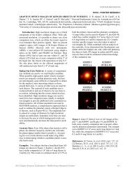
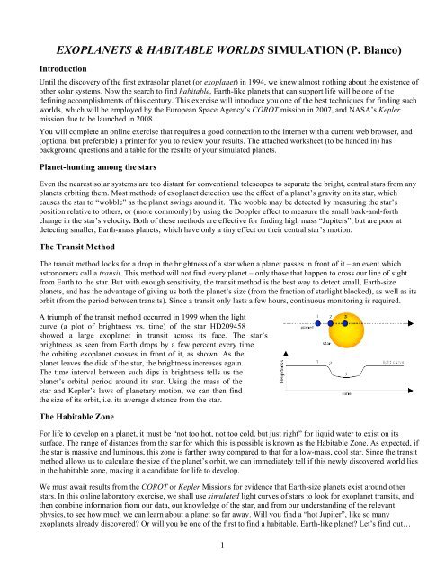
A triumph of the transit method occurred in 1999 when the light
curve (a plot of brightness vs. time) of the star HD209458
showed a large exoplanet in transit across its face. The star’s
brightness as seen from Earth drops by a few percent every time
the orbiting exoplanet crosses in front of it, as shown. As the
planet leaves the disk of the star, the brightness increases again.
The time interval between such dips in brightness tells us the
planet’s orbital period around its star. Using the mass of the
star and Kepler’s laws of planetary motion, we can then find
the size of its orbit, i.e. its average distance from the star.
The Habitable Zone
For life to develop on a planet, it must be “not too hot, not too cold, but just right” for liquid water to exist on its
surface. The range of distances from the star for which this is possible is known as the Habitable Zone. As expected, if
the star is massive and luminous, this zone is farther away compared to that for a low-mass, cool star. Since the transit
method allows us to calculate the size of the planet’s orbit, we can immediately tell if this newly discovered world lies
in the habitable zone, making it a candidate for life to develop.
We must await results from the COROT or Kepler Missions for evidence that Earth-size planets exist around other
stars. In this online laboratory exercise, we shall use simulated light curves of stars to look for exoplanet transits, and
then combine information from our data, our knowledge of the star, and from our understanding of the relevant
physics, to see how much we can learn about a planet so far away. Will you find a “hot Jupiter”, like so many
exoplanets already discovered? Or will you be one of the first to find a habitable, Earth-like planet? Let’s find out…
1

Transit Method Simulation: Procedure
From a current web browser, go to one of the websites given on the next page to start running the simulation, which
guides you through 8 pages of information and calculations.
Page 1: Read the Introduction on this web page – you will have to answer questions later. Then select the
“Simulation” link, and you will be directed to page 1 of the exercise, which shows a patch of sky with stars, numbered
1 through 8. Pick a star to analyze. You will see a plot of the star’s “light curve” (brightness as a function of time). If
the star has a planet whose orbit causes transits along our line-of-sight, you will see periodic “dips” in this plot. As
carefully as you can (here is where a printer will help), estimate the Period P of the planet’s orbit.
Page 2: A star’s “spectral type” (which is related to its mass, temperature, and power output) is given by a letternumber
code. For instance, our star is a “G5”, where as a lower mass star could be a “K2”. (The letter sequence from
high- to low- mass is OBAFGKMRN, remembered as “Oh Be A Fine Guy/Girl Kiss Me Right Now!”). From the
table given, look up and enter the star’s mass. orbit. Select Calculate and the program use Kepler’s 3 rd law (P 2 =a 3 /M)
to calculate the size of the planet’s orbit. You’re now on your way to finding out more about the [simulated] exoplanet
you have discovered!
Page 3: Plotting your star’s mass vs. your planet’s orbital distance, you can determine whether your new planet falls
within the central star’s Habitable Zone. This is the zone generally considered to be “not too hot, not too cold, but just
right” for liquid water to exist in the presence of at atmosphere – conditions which are thought to be essential for life
to develop. You may find it easier to accomplish this task by printing a paper copy of the plot provided.
Page 4 uses the central star’s radius and temperature are to estimate your exoplanet’s temperature at its orbital
distance (assuming a circular orbit). Here the temperatures are expressed in Kelvin above absolute zero. So, for
example, 0°C = 32°F = 273 K. Planets with temperatures around 300 K could be considered “habitable”. Obviously, a
planet’s temperature will increase with the star’s temperature and size, but decrease with orbital distance. Luckily for
you, the computer does most of the work once you have provided the information. Look up the star’s radius and
temperature for its spectral type from the tables provided, enter the information and select Calculate.
Page 5 is an “automatic” calculation of your planet’s physical size, based on the drop in light output as it transits the
face of the star. Simply select Calculate, but be sure to read the information presented on this page.
Page 6 uses two separate “models” of a planet’s density based on the planets in our solar system, to estimate the
possible mass of the new exoplanet. (Unlike the “stellar wobble” methods of detection, the transit method does not
give us a planet’s mass directly). One model uses your exoplanet’s radius, the other uses its distance from the star –
both of which have already been calculated. From each of the curves presented for each model, estimate your planet’s
density, and select Calculate. Do not be concerned if the two mass estimates are vastly different! With more
exoplanets being found by various methods, we hope that soon we can construct better models of solar system
contents, instead of just relying on our own (possibly atypical) solar system.
Page 7 concludes the simulation with an “automatic” calculation of the probability of detecting such a planet. Since
planetary systems will only orbit in the plane containing our line-of-sight by chance, the Kepler mission will only
detect a fraction of all exoplanets. But by observing many stars, we should expect success in a significant number of
cases.
Page 8 presents a summary of all the parameters you have calculated, which you can use to complete the summary
table on the worksheet.
NOW REPEAT THE SIMULATION WITH A DIFFERENT STAR. Note the some of the stars do not have
detectable planets in this exercise, so if this is the case, make a note of the star’s ID# and select another. Happy planet
hunting!
2

The simulation website is at:
http://www.bridgewater.edu/~rbowman/ISAW/Transit-1.html
If for some reason this website is not accessible, an alternate site to run the simulation is:
http://www.astro.lsa.umich.edu/Academics/Undergrad/Labs/exoplanets/Transit-1.html
SUMMARY TABLE for the two simulated exoplanets
EXOPLANET SYSTEM INFORMATION 1st simulation 2 nd simulation
Star ID (#1-8), and spectral type (e.g. A0, G5, K2)
Star’s mass M Star (solar masses)
Star’s radius R Star (solar radii)
Star’s surface temperature T Star (Kelvin)
Notes:
Planet’s measured orbital Period P (yr)
Planet’s orbital size (semi-major axis) a (A.U.)
Planet orbits in the Habitable Zone? (Yes or No)
Planet’s estimated surface temperature T P (K)
Planet’s radius R P (Earth radii)
Planet’s mass range (in Earth masses, min. to max.)
e.g. “1.3 – 2.8”
Probability of discovery (%)
• Some stars in this exercise do not have exoplanets that produce a good light curve with a measurable period
between transits. If you select one of these, make a note of its ID number below the table, then pick another star.
• Boxes containing the words “automatic” are not for data entry. After you have filled the other boxes with the
necessary data, select Calculate and the computer will update these boxes (and its ongoing summary of results, see
below).
• In order to answer the questions properly, you will need to READ the background information on each page of
the simulation. Much of this information is given below the Next button, so scroll down to read it (or print each page).
• The simulation keeps track of any calculations made, so if you need a piece of information about the star, or the
exoplanet, look for it in the ongoing summary at the top of the web page. You can also record your results in the
Summary Table above as you progress through the simulation, or simply copy the numbers from the final page of the
exercise.
3

Exoplanets Simulation Worksheet. TO BE HANDED IN! NAME: _________________
1. Briefly, describe in words the transit method of detecting an extrasolar planet.
2. From the period P (in Earth years) of a planet’s orbit around a star of mass M Star solar masses, we can use Kepler’s
3 rd law P 2 =a 3 /M Star to find the size of the planet’s orbit a in Astronomical Units (A.U.). If we see a planet orbiting a
star of mass M Star = 2.5 solar masses with an orbital period P=3.0 years, what is the size of its orbit?
Size of orbit a = ___________ A. U.
3. What is meant by the Habitable Zone around a star? From the graph shown on page 3 of the simulation: would you
expect the habitable zone for a low-mass star to be closer in, farther out, or the same distance from the star, compared
to the habitable zone around our Sun? Give a reason for your answer.
4. The transit method gives us a planet’s size radius R, but not its mass. For that, we also need the planet’s average
density. Suppose a planet has a radius R = 5.6 ×10 6 m. If its average density is 4200 kg/m 3 , calculate the planet’s mass:
(a) in kg, and (b) in Earth masses. (Volume of sphere = 4 / 3 πR 3 , Earth’s mass = 6.0×10 24 kg)
a. Planet mass in kg: ____________ kg. b. Planet mass in Earth masses: __________ M Earth
Show your calculation work here:
4