Inverse Distance Weighting for Extrapolating Balloon ... - Nexo

Inverse Distance Weighting 

for Extrapolating Balloon-Directivity-Plots 

Joerg Panzer 

NEXO 

joerg.panzer@nexo.fr 

Daniele Ponteggia 

Audiomatica 

dp@audiomatica.com 

Presented at the AES 131th Convention, New York, 2011 

Abstract 

This paper investigates an extrapolation for missing directivity-data in connection with Balloon-Plots. Such 

plots display the spherical directivity-pattern of radiators and receivers in form of contoured sound pressure 

levels. Normally the directivity-data are distributed evenly so that at each point of the display-sphere there 

would be sufficient data-points. However, there are circumstances where we want to display data that are 

not evenly distributed. For example, there might be only available the horizontal and vertical scans. The 

proposed Inverse Distance Weighting method is a means to extrapolate into these gaps. This paper explains 

this method and demonstrates some examples. 

1 INTRODUCTION 

The radiation characteristic of electro-acoustic devices 

can be measured or simulated by sampling over a sphere 

of a given radius around the device under test. 

Usually the sampling is carried out in spherical coordinates 

on a regular angular grid, as described in [1]. 

Once data are collected, the data-set is graphically represented 

with the help of so called balloon-plots. These 

plots are in the form of contour plots over a spherical surface 

or as surfaces in spherical coordinates where the radius 

is proportional to the gain of the device along the 

pointed direction. 

It may happen that, due to the complexity of measurement 

infrastructure or non-regular sampling over the 

spherical surfaces, that there is need to extrapolate data 

from a reduced or incomplete set of measurement points. 

On the sphere, therefore, there might be gaps large 

enough that we do not know the values, hence the usage 

of the term “extrapolate” in the sense of [2]: 

“In mathematics, extrapolation is the 

process of constructing new data points. It 

is similar to the process of interpolation, 

which constructs new points between known 

points, but the results of extrapolations are 

often less meaningful, and are subject to 

greater uncertainty. It may also mean extension 

of a method, assuming similar methods 

will be applicable. ...” 

Beside the gaps, dense data might be available. For 

example a common case is the extrapolation from measurements 

done on horizontal and vertical scan-lines 

only. 

Because on the sphere any point is naturally “surrounded” 

by other points, we could perform any of the 

interpolation-schemes in order to obtain an intermediate 

value [3][4]. However, in this paper, we would like to 

draw attention to a particular scheme, which is straightforward 

to apply and which can be used for interpolation 

as well as for extrapolation problems. It seems to cope 

well also with anisotropic distribution of points. The approach 

is based on [5]. We have adapted it for spherical 

coordinates and we call it Inverse Distance Weighting 

(IDW) as described in section 2.1.2. 

In the first part of this paper we investigate the extrapolation 

applied to a canonical test-function on an 

anisotropic grid. For comparisons two approaches are 

shown: 1) Decomposition with Spherical Harmonics. 

2) The Inverse Distance Weighting. The first part also 

explains the Inverse Distance Weighting. 

The second part demonstrates the application of the 

Inverse Distance Weighting method to a set of measurement 

curves. 

2 TEST FUNCTION 

The “SincSinc”-function features the directivity of a rectangular 

piston in an infinite baffle [6]. 

( ) ( ) 

Lx 

D (k x , k y ) = sinc 

2 · k Ly 

x · sinc 

2 · k y 

1

Panzer, Ponteggia 

IDW for Extapolating Balloon-Plots 

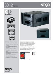
Figure 1: Test-function at 5 kHz mapped on a mesh of regular polar-scan-lines with an angular resolution of 5 deg. To the 

right is shown the projection of the levels along the ring at 45 deg onto a polar-plot. 

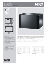
Figure 2: Spherical grids. 

with k x = k·cos (ϕ)·sin (θ), k y = k·sin (ϕ)·sin (θ), 

k = ω/c, ω is angular frequency, c is speed of sound, ϕ 

is the azimuthal and θ is polar angle in spherical coordinates. 

L x and L y are the dimensions of the rectangle. 

For all examples the test-function is used with following 

values: L x =0.2 m, L y =0.1 m, c= 343 m/s. A frequency 

f = 5 kHz is used. 

The highest angular resolution of any balloon-mesh 

is 5 deg. All contours display a range of 50 dB in steps of 

3 dB. 

The SincSinc-function turns out to be a good testfunction 

for checking extrapolation schemes for radiation 

problems, because it features typical radiation patterns including 

marked interferences (figure 1). 

Note, the data-set has been rotated by 2.5 deg about 

the x-, y- and z-axis in order to provide a simple regularization 

for following analysis. With the help of the slight 

shift we make sure that target points do not coincide with 

source points and thus true interpolation is always performed. 

2.1 Extrapolation Example 

In the following we want to demonstrate the basic problem 

by constructing an example, which would makes necessary 

extrapolation. The idea is to use the SincSincfunction 

as an example and to calculate values on a non 

regular grid on the sphere. 

An anisotropic grid could be constructed in the following 

way. To the left of figure 2 we have the regular 

grid with 5 deg angular resolution. The mesh in the center 

is anisotropic and provides points at 5 deg resolution 

in polar direction and 30 deg resolution in azimuthal direction, 

hence there are wide gaps circumferential. The 

right plot, finally, pictures the extreme case, where there 

is a dense distribution of points on vertical and horizontal 

scan-lines but naught in between. 

The idea is to investigate how two selected interpolation 

schemes cope with the rarefied distributions. Because 

we know how the function should appear, if sampled 

properly, we can compare the pictures of the balloon 

plot and a selected mapping of a polar-plot (along 

the dark arc) to the original plots as shown in figure 1. 

2.1.1 Spherical Harmonics 

Intuitively a promising interpolation scheme should be 

holistic, which means it would take into account all available 

points in order to magically fill the gaps. Is there a 

function, which by nature behaves like a “radiator”? If 

2



Figure 3: Extrapolation with Spherical Harmonics. 

we take many of such functions and weight each of these 

in such a way that the sum-total satisfies known-values on 

the sphere, then it should also give reasonable values for 

the unknown territory. These functions are called Spherical 

Harmonics or Multipole Expansion [6]. 

Spherical Harmonics is the natural mode-set of a 

sphere. In principal any regular distribution of values on 

a sphere can be assembled from a spectrum of Spherical 

Harmonics, similar to Fourier and polynomial interpolation 

in Cartesian coordinates. 

The text-book implementation of modal decomposition 

in Spherical Harmonics works fine as long as each 

mode gets sufficient data-points to adjust itself. This is 

one of the reasons why we have added a little rotation to 

3



Figure 4: Extrapolation with IDW. 

the original data-set, in order to avoid nodal lines of the 

modes to fall on peculiar scan-lines of the data-set. 

For 5/5 deg: The first row of the picture-table 3 is 

a decomposition with 20·20-modes on a regular 5 deg 

mesh. The decomposition compares well to the original. 

For 5/30 deg: The second row shows the decomposition 

of an anisotropic grid. The algorithm turned out to 

be stable only up to 6·6 modes. Compared to the original, 

the balloon-contours and the polar-curve are quite different. 

However, for a “reach into the unknown” the result 

may be considered not too bad. First, the overall pattern 

is reproduced in level. Second, the Spherical Harmonics 

yields typical interference patterns of a radiator, which 

other general extrapolation schemes may not be able to 

4



produce. 

For 5/90 deg: The modal decomposition algorithm 

turned out to be unstable for any mode beyond 2·2 

(dipoles). However, the result is an omni-directional 

mean-value. 

2.1.2 Inverse Distance Weighting 

The Inverse Distance Weighting method (IDW) is a sort 

of mean-value forming approach for calculating a value 

at any point on the sphere by taking into account the contribution 

of all original points. 

f (P ) = 

∑ 

i 

d −u 

i 

∑ 

i 

d −u 

i 

f (P ) = z i | di→0 

· z i 

with f(P ) a value anywhere on the sphere at point P . 

z i is a value from the original data-set at point D i . The 

function d i is the surface-distance on the sphere between 

vectors P and D i : 

d i = arccos (P · D i ) 

For Inverse Distance Weighting the factor u ≥ 1. 

Typically u = 2...5. For the above examples u = 3 

is used. For interesting details see [5]. If d i = 0 then 

we substitute the original value z i at point D i . It turned 

out that the algorithm works better if only points from a 

hemisphere are used with: 

P · D i > 0 

Thus, each data-point contributes according to the inverse 

of its distance. Data-points, which are close to P 

provide a strong influence, and data-points further away 

contribute less. Naturally, the IDW provides a very stable 

extrapolation as long as u ≥ 1. However, as the weightfunction 

does not provide oscillations there are no additional 

interferences produced, which in turn yields the resulting 

values of the extrapolation often to be too optimistic. 

Or, in other words, the values further away from 

the original data-set turn out to be too high compared to 

the regular sampled version. 

Figure 4 provides levels as contours on the balloon 

surface and polar-plots of the Inverse Distance Weighting 

method. As in the previous example the original dataset 

is the SincSinc-function (figure 1) rotated by 2.5 deg 

about x-, y- and z-axis. The rotation is applied in order 

to trigger the IDW for all cases. All extrapolations are 

performed with u = 3. 

For 5/5 deg: The first row shows the application of 

the IDW on the regular grid. Because of the rotation by 

2.5 deg the IDW provides interpolated values. The results 

compare well to the pictures of the original function. 

Some spatial smoothing is present. 

For 5/30 deg: The second row shows the result of 

the IDW for original points distributed on an anisotropic 

grid. The pattern of the contours is different compared 

to the original balloon, however, the main features are 

maintained. The response obviously appears strongly 

smoothed as can be seen also in the polar-plot. 

For 5/90 deg: The last row displays the extreme 

case, where the original function is provided only on two 

scan-lines. Interestingly the balloon contours still display 

some of the main features of the directivity of a rectangular 

piston. However, as already stated, the level in the 

extrapolated regions turn out to be too high. This is understandable 

because the original function provides interference 

whereas the IDW does not. 

Compared to the Spherical Harmonic approach the 

IDW seems more stable and easy to adjust. During experiments 

the Spherical Harmonic approach often failed, 

needed special regularization and asked for a careful adjustment 

of the number of modes. The IDW on the other 

hand always yields a meaningful result, however, often 

blurred and too optimistic. 

3 MEASUREMENT 

The measurement of a loudspeaker 3D directivity, as described 

in [1], requires the loudspeaker impulse response 

to be sampled with a 5 degree resolution “equi-angular” 

spherical pattern. This means a total of 2664 measurement 

points [7]. 

Among the different approaches to acquire the 3D 

measurement set we may: use multiple microphones, 

move one or more microphones around the loudspeaker, 

use a single fixed microphone coupled with a mechanical 

system to orient the loudspeaker towards a given direction 

or any mix of the above. It is outside the scope of 

this paper to enter into the details of 3D measurements. 

We would like to point out here the complexity of such 

kind of setup, both in terms of needed hardware and time. 

A simpler and more cost-effective alternative is to 

sample the sphere over only a few scan-lines. Using a 

single fixed microphone and a single turntable (or equivalent) 

it is easily possible to sample the loudspeaker response 

over the horizontal and vertical scan-lines. This 

can be done by placing the loudspeaker in vertical and 

horizontal position on the turntable, the rotation of the 

turntable corresponds to an apparent rotation of the microphone 

around the loudspeaker. 

In this case the full balloon response has to be extrapolated 

from the available data. We will compare here the 

results of 5 degrees full-balloon measurements with an 

extrapolation made with the IDW method. 

Before showing the results of real world examples, 

we need to introduce another graphical representation of 

the 3D directivity in the form of a color-map as rectangular 

projection of the sphere: the two spherical coordinates 

angles ϕ and θ are projected on the x- and y- axes, while 

the sound pressure level is represented by a color shade 

(see figure 5). Despite the distortion introduced by such 

projection, this allows for a simple representation of the 

5



Figure 5: Color-map plot: directivity balloon is projected on a plane. 

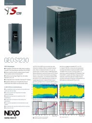
Figure 6: Driver on exponential horn balloon at 8 kHz: (left-top) 5 degree measured, (right-top) IDW extrapolation, 

(bottom) absolute error. 

difference between 5 degrees 3D balloon measurement 

and data extrapolation made with the IDW method. 

We will report here two different case studies: a 

1 inch compression driver on a 90x60 exponential horn, 

and a small bookshelf 2-way sealed loudspeaker box. 

Throughout these examples u = 3 has been used for the 

IDW extrapolation and data has been smoothed by third 

octave bands. 

3.1 Compression driver on exponential 

horn 

The driver-horn assembly has been measured in 3D using 

two computer controlled turntables, with an angular 

resolution of 5 degrees. Since the source has a symmetry 

along the vertical and horizontal planes, only a quarter of 

a sphere has been sampled and data has been then mirrored. 

Figure 6 (left-top) shows the measured balloon plot 

(in this plot the surface is distorted in such a way that the 

radius of the sphere is proportional to the sound pressure 

level) of the driver at 8 kHz frequency band, where the 

effect of the rectangular aperture is clearly visible. In the 

same figure 6 (right-top) the balloon extrapolated from 

horizontal and vertical scan-lines using the IDW method 

is shown. 

The absolute error in dB between measured and data 

extrapolated is shown in the bottom row of figure 6 as a 

color-map plot. 

While the absolute error is not small, the overall balloon 

shape is not affected, as previously found with the 

sincsinc test function. 

3.2 Small 2-way loudspeaker box 

The 2-way box has been measured in 3D using the same 

setup as above. Due to the horizontal symmetry only half 

sphere has been sampled and then data mirrored. 

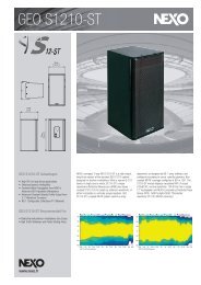
This loudspeaker exhibits an interference pattern between 

the two drivers at the crossover frequency. The 

interference can be seen in the 3.15 kHz one third frequency 

band measured balloon (figure 8 (left-top)). 

Figure 8 (mid-top) illustrates the balloon extrapolated 

from horizontal and vertical scan-lines using the 

IDW method. A color-map plot of the absolute error 

of the IDW extrapolation using the above scan lines is 

6



Figure 7: Horizontal, Vertical and Equatorial Scan-Lines. 

Figure 8: 2-Way loudspeaker at 3.15 kHz: (left-top) 5 degree measured, (mid-top) IDW extrapolation H+V, (right-top) 

IDW extrapolation H+V+E, (left-bottom) absolute error H+V, (right-bottom) absolute error H+V+E. 

in figure 8 (left-bottom). Here again, while the balloon 

presents quite a complex behavior featuring multiple 

side-lobes, the overall shape is kept and side-lobes 

are present, albeit attenuated. 

The error of the IDW extrapolation can be reduced using 

more scan-lines. We will propose here a very simple 

setup to collect an additional scan-line that, in an analogy 

with earth science, we call “equatorial” (figure 7). 

The proposed setup uses a single turntable and a single 

fixed microphone, as in the case of horizontal and vertical 

scan-lines. In order to collect the equatorial scan-line, the 

loudspeaker under test has to be placed on the turntable 

facing up (pointing towards the ceiling). 

The balloon plot of the data extrapolated with IDW 

method using horizontal, vertical and equatorial scan-line 

is presented in figure 8 (right-top) and the error is shown 

as color-map plot in the same figure (right-bottom). The 

presence of the “equatorial” data helps to reduce the error, 

while the required additional measurement effort is 

minimum. 

4 CONCLUSIONS 

This paper reports on the investigation of the application 

of the Inverse Distance Weighting method for extrapolating 

incomplete 3D directivity data. 

The IDW is not a substitute for the complete data-set 

as can clearly been seen by the investigation of the canonical 

SincSinc function and by the error-maps of measurements 

done. However, the IDW can provide rough estimates 

for the unknown areas even under the extreme case, 

where only a horizontal and vertical scan-line is available. 

In any case the IDW provides bounded results and is easy 

to apply. 

As most measurement setups go along scan-lines it 

seems beneficial in this context to measure the device un- 

7



der test also equatorial. 

Future research will investigate refinements of the 

IDW and will look into other possibilities of extrapolating 

the balloon-plot. 

5 AKNOWLEDGEMENTS 

The authors sincerely acknowledge the companies 

NEXO S.A. (www.nexo.fr) and Audiomatica (www. 

audiomatica.com) for support of this paper. 

References 

[1] AES Standard, “Sound source modeling - loudspeaker 

polar radiation measurements”, AES56- 

2008. 

[2] Wikipedia, “Extrapolation”, https: 

//secure.wikimedia.org/wikipedia/ 

en/w/index.php?title= 

Extrapolation&oldid=438224623 (accessed 

August 8, 2011). 

[3] Renka, R., “Interpolation of data on the surface of 

a sphere and triangulation and interpolation at arbitrary 

distributed points in the plane”, ACM Trans. 

Math. Softw 10, 4 (Dec 1984). 

[4] Buss, S., Fillmore, J., “Spherical averages and applications 

to spherical splines and interpolation”, 

ACM Trans. Graph., 20, 2 (April 2001). 

[5] Shepard, D., “A two-dimensional interpolation 

function for irregular-spaced data”, ACM Proc. Nat. 

Conf. 1968. 

[6] Williams, E., “Fourier acoustics”, Academic Press, 

1999. 

[7] Ponteggia, D., “AN-002, Automated Balloon 

Measurements Using CLIO 10”, http: 

//www.audiomatica.com/download/ 

appnote_002.pdf, Audiomatica, 2009 

8

Inverse Distance Weighting for Extrapolating Balloon ... - Nexo

Create successful ePaper yourself

Delete template?

Save as template?