Non-Euclidean geometry and the Robertson-Walker metric
Non-Euclidean geometry and the Robertson-Walker metric
Non-Euclidean geometry and the Robertson-Walker metric

Create successful ePaper yourself
Turn your PDF publications into a flip-book with our unique Google optimized e-Paper software.
Astronomy 401<br />
Lecture 28<br />
<strong>Non</strong>-<strong>Euclidean</strong> Geometry <strong>and</strong> <strong>the</strong> <strong>Robertson</strong>-<strong>Walker</strong> Metric<br />
We’ve been talking about different scenarios for <strong>the</strong> evolution of <strong>the</strong> universe: open, flat or closed, depending<br />
on <strong>the</strong> density of mass <strong>and</strong> energy. This is very closely related to <strong>the</strong> <strong>geometry</strong> of <strong>the</strong> universe, which is<br />
described by general relativity. To underst<strong>and</strong> <strong>the</strong> curvature of <strong>the</strong> universe, we need to consider some of<br />
<strong>the</strong> principles of non-<strong>Euclidean</strong> <strong>geometry</strong>.<br />
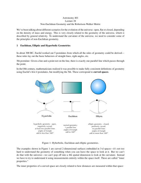
1 <strong>Euclidean</strong>, Elliptic <strong>and</strong> Hyperbolic Geometries<br />
In about 300 BC, Euclid worked out 5 postulates from which all <strong>the</strong> rules of <strong>geometry</strong> could be derived—<br />
<strong>the</strong>se rules lay out <strong>the</strong> basic behaviors of straight lines, right angles, etc.<br />
5th postulate: Given a line <strong>and</strong> a point not on <strong>the</strong> line, <strong>the</strong>re is exactly one parallel line which passes through<br />
<strong>the</strong> point.<br />
In <strong>the</strong>18th century, ma<strong>the</strong>maticians realized it was possible to make fully consistent definitions of <strong>geometry</strong><br />
using Euclid’s first 4 postulates, but modifying <strong>the</strong> 5th. These correspond to curved spaces.<br />
hyperbolic <strong>geometry</strong> - open,<br />
negatively curved:<br />
at least two parallel lines<br />
angles of triangle<br />
add to less than 180 O<br />
normal <strong>geometry</strong>:<br />
1 parallel line<br />
angles of triangle<br />
add to 180 O<br />
elliptic <strong>geometry</strong> - closed,<br />
positively curved:<br />
no parallel lines<br />
angles of triangle<br />
add to more than 180 O<br />
Figure 1: Hyberbolic, <strong>Euclidean</strong> <strong>and</strong> elliptic geometries.<br />
The examples shown in Figure 1 are curved 2-dimensional surfaces embedded in 3-d spaces—it’s not too<br />
hard to underst<strong>and</strong> <strong>the</strong> <strong>geometry</strong> of something when you can leave <strong>the</strong> space to look at it. But we can’t<br />
do that with <strong>the</strong> universe—we can’t pop off into a 4th spatial dimension to look at <strong>the</strong> curvature. Instead<br />
we have to try to underst<strong>and</strong> it using measurements entirely within <strong>the</strong> space itself. These are called “inner<br />
properties.”<br />
The inner properties of a curved space are closely related to how distances are measured within that space:
• On a flat <strong>Euclidean</strong> plane, a circle has circumference C = 2πr.<br />
• On a sphere of radius R, <strong>the</strong> radius of <strong>the</strong> circle r = Rθ, but <strong>the</strong> circumference is<br />
C = 2π(R sin θ) (1)<br />
( ) sin θ<br />
= 2πr<br />
(2)<br />
θ<br />
< 2πr (3)<br />
So, an observer on <strong>the</strong> surface of a sphere could measure <strong>the</strong> radius <strong>and</strong> circumference of a circle, <strong>and</strong><br />
deduce that <strong>the</strong>y were living in a positively curved world.<br />
R sin θ<br />
r<br />
θ<br />
R<br />
Figure 2: A circle on <strong>the</strong> surface of a sphere.<br />
• Similarly, in a negatively curved space, C > 2πr.<br />
2 Measuring distances <strong>and</strong> <strong>the</strong> <strong>Robertson</strong>-<strong>Walker</strong> <strong>metric</strong><br />
These differences in “big” distances must reflect differences in <strong>the</strong> infinitesimal distances from which <strong>the</strong>y<br />
are made up:<br />
∫<br />
L = dl (4)<br />
In <strong>Euclidean</strong> space, <strong>the</strong> distance between two points is<br />
L 2 = x 2 + y 2 (5)<br />
or equivalently in polar coordinates,<br />
We express infinitesimal separations similarly:<br />
L 2 = r 2 . (6)<br />
(dl) 2 = (dx) 2 + (dy) 2 (7)<br />
2
y<br />
dy<br />
dl<br />
dx<br />
r<br />
r dɸ<br />
dl<br />
dr<br />
dɸ<br />
x<br />
Figure 3: Infinitesimal distances.<br />
or in polar coordinates<br />
(dl) 2 = (dr) 2 + (r dφ) 2 (8)<br />
We call <strong>the</strong> rule for how distances are measured in a space <strong>the</strong> <strong>metric</strong>, e.g. dl 2 = dr 2 + r 2 dφ 2 is <strong>the</strong> <strong>metric</strong><br />
for a flat <strong>Euclidean</strong> space.<br />
We can define a different <strong>metric</strong> for a different <strong>geometry</strong>. For example, <strong>the</strong> distance between any two points<br />
on <strong>the</strong> surface of a sphere of radius R is given by<br />
(dl) 2 = (R dθ) 2 + (r dφ) 2 , (9)<br />
with radial coordinate r <strong>and</strong> angular coordinates θ <strong>and</strong> φ. Since r = R sin θ, dr = R cos θ dθ, <strong>and</strong><br />
R dθ =<br />
dr<br />
cos θ =<br />
R dr √<br />
R 2 − r 2 =<br />
dr<br />
√<br />
1 − r 2 /R 2 (10)<br />
(since r = R sin θ <strong>and</strong> sin 2 θ + cos 2 θ = 1). So our <strong>metric</strong> for distance on <strong>the</strong> surface of <strong>the</strong> sphere is<br />
(<br />
) 2<br />
(dl) 2 dr<br />
= √ + (r dφ) 2 . (11)<br />
1 − r 2 /R 2<br />
For a general two-dimensional surface with curvature<br />
K ≡ 1 R 2 , (12)<br />
<strong>the</strong> <strong>metric</strong> is<br />
( )<br />
(dl) 2 dr 2<br />
= √ + (r dφ) 2 . (13)<br />
1 − Kr 2<br />
We generalize this to three dimensions:<br />
( )<br />
(dl) 2 dr 2<br />
= √ + (r dθ) 2 + (r sin θ dφ) 2 . (14)<br />
1 − Kr 2<br />
K is now <strong>the</strong> curvature of <strong>the</strong> 3-d space. Note that as K → 0 or r → 0, <strong>the</strong> space acts <strong>Euclidean</strong>.<br />
3
Next we substitute r = a(t)x, where a(t) is <strong>the</strong> scale factor <strong>and</strong> x is <strong>the</strong> comoving coordinate:<br />
[( )<br />
(dl) 2 = a 2 dx 2 ]<br />
(t) √ + (x dθ) 2 + (x sin θ dφ) 2<br />
1 − Kx 2<br />
(15)<br />
Finally, we are measuring distances in spacetime, not just space. By distance, we mean <strong>the</strong> proper distance<br />
between two spacetime events that occur simultaneously, according to an observer. The spacetime <strong>metric</strong> is<br />
(ds) 2 = (c dt) 2 − (dl) 2 . (16)<br />
Therefore, we have<br />
[( )<br />
(ds) 2 = (c dt) 2 − a 2 dx 2 ]<br />
(t) √ + (x dθ) 2 + (x sin θ dφ) 2<br />
1 − Kx 2<br />
(17)<br />
This is <strong>the</strong> <strong>Robertson</strong>-<strong>Walker</strong> <strong>metric</strong>, <strong>and</strong> it is used to determine <strong>the</strong> spacetime interval between two events<br />
in any homogeneous, isotropic space (both positively <strong>and</strong> negatively curved, though we only showed it for<br />
<strong>the</strong> simplest, spherical case here).<br />
Also note that <strong>the</strong> curvature parameter K is <strong>the</strong> K that appears in <strong>the</strong> Friedmann equation,<br />
[(ȧ(t)<br />
a(t)<br />
) 2<br />
− 8π 3 Gρ ]<br />
a 2 (t) = −Kc 2 . (18)<br />
In our Newtonian derivation of this equation, K referred to <strong>the</strong> total energy of <strong>the</strong> universe, but when this<br />
equation is derived from general relativity, K is <strong>the</strong> curvature constant defined above. Thus if K = 0,<br />
<strong>the</strong> space is <strong>Euclidean</strong>, i.e. flat. If K > 0, 1/ √ K can be interpreted as <strong>the</strong> radius of curvature of <strong>the</strong><br />
three-dimensional space; <strong>the</strong> two-dimensional analogy is <strong>the</strong> surface of a sphere. If K < 0, <strong>the</strong> space is<br />
hyperbolic—<strong>the</strong> open <strong>geometry</strong> shown in Figure 1.<br />
4