Exact geometric optics in a Morris-Thorne wormhole spacetime

PHYSICAL REVIEW D 77, 044043 (2008)
Exact geometric optics in a Morris-Thorne wormhole spacetime
Thomas Müller
Visualisierungsinstitut der Universität Stuttgart, Nobelstrasse 15, 70569 Stuttgart, Germany
(Received 17 December 2007; published 26 February 2008)
The simplicity of the Morris-Thorne wormhole spacetime permits us to determine null and timelike
geodesics by means of elliptic integral functions and Jacobian elliptic functions. This analytic solution
makes it possible to find a geodesic which connects two distant events. An exact gravitational lensing, an
illumination calculation, and even an interactive visualization become possible.
DOI: 10.1103/PhysRevD.77.044043 PACS numbers: 04.20. q, 04.20.Jb
I. INTRODUCTION
The notion of a wormhole was first introduced in 1962
by John Wheeler [1] who reinterpreted the Einstein-Rosen
bridge [2] as a connection between two distant places in
spacetime with no mutual interaction. However, he realized
together with Robert Fuller [3] that this Schwarzschild
wormhole cannot be traversed even by a single particle. In
1988, Michael Morris and Kip Thorne [4] presented the
most simple metric which serves as a wormhole that could
in principle be traversed by human beings. [5] From that
time on, there are a lot of publications which suggest new
types of wormholes, see e.g. [7–13]. But all of them have in
common that they violate the weak energy condition. For a
detailed discussion see, for example, Visser [14].
One of the difficulties in curved spacetimes is to find a
geodesic which connects two distant events. The common
astrophysical application is the gravitational lensing of a
distant object by means of a very massive object like a
galaxy or a black hole. Here, the null geodesics connecting
the distant object with the observer are searched. In the
case of the Schwarzschild spacetime, Frittelli et al [15]
construct the exact lens equation. A short discussion of
gravitational lensing by wormholes can be found in Cramer
et al [16] or Nandi et al [17]. A detailed review of gravitational
lensing in curved spacetime with several examples
is given by Perlick [18].
In general, there is no mathematical procedure which
could find a geodesic in a four-dimensional spacetime
connecting two events in a reasonable time. The shooting
method [19] might be applicable in a two-dimensional
problem. Another possibility would be the precalculation
and tabulating of geodesics. But the disadvantage of this
method is the extreme amount of data which must be
searched. Furthermore, the ambiguity which appears
when connecting two events drastically complicates the
solution. The only practical method is, so far as it exists, to
use the analytic solution of the geodesic equation.
In contrast to the Schwarzschild case as shown by Čadež
and Kostić [20], the analytic solution of the geodesic
equation in the Morris-Thorne (MT) spacetime is quite
*Thomas.Mueller@vis.uni-stuttgart.de
straightforward. Starting from the Lagrangian equations
for the MT metric, one immediately gets the orbital equation
for a geodesic as an elliptic integral of the first kind in
standard form. Like in the Schwarzschild case, one has to
make a distinction where the null geodesic starts and ends.
However, in the MT case, we do not have to deal with
complex arguments or modules in the elliptic integrals
which definitely simplifies the calculations.
The aim of this article is to derive the exact analytic
solution of the geodesic equation in the MT spacetime and
to show its relevance for connecting two events with a
lightlike geodesic. The most prominent application is the
determination of the exact gravitational lens equation,
compare Perlick [21]. In contrast to Perlick, we will formulate
the lens equation in terms of elliptic integral functions
which makes the orbits of the geodesics more
transparent. A second application might be the visualization
of the MT spacetime from a first-person’s point of
view. By means of objects in motion or at rest some aspects
of the topology and the inner geometry of the spacetime
become visible. The importance of visualization to get a
better insight of special and general relativity is demonstrated,
for example, in [22–25]. A visualization of the
Morris-Thorne wormhole is given by the author [26]. In
general, the ray tracing method is used where a null geodesic
is traced back in time from the observer to the point
of emission to render the view of an observer. But this
method is quite time consuming and is not capable of
including a correct illumination of the scenario. This limitation
can be bypassed with the exact solution of the
geodesic equation. Finally, an interactive visualization by
means of today’s fully programmable graphics processing
units (GPUs) becomes possible.
In Sec. II we give a short introduction to the Morris-
Thorne spacetime and explain the topological structure by
means of an embedding diagram. For the initial conditions
of the geodesics we take the perspective of a local observer
whose reference frame is represented by a local tetrad. This
is a more intuitive approach than the use of angular momentum
and longitude of periapsis. The main part of this
article concerns with the analytic solution of the geodesic
equation which will be discussed in Sec. III. As we will
see, the orbits of lightlike, timelike, and spacelike geo-
1550-7998=2008=77(4)=044043(11) 044043-1 © 2008 The American Physical Society

THOMAS MÜLLER PHYSICAL REVIEW D 77, 044043 (2008)
desics in the Morris-Thorne spacetime are all equal. As a
upper universe
first application, Sec. IV explains the determination of
distance and throat size by means of a flash of light. In
Sec. V we show how two arbitrary points can be connected
by a lightlike geodesic. This enables us to determine the
exact lens equation in Sec. VI. Finally, we can easily show
in Sec. VII how wave fronts propagate in the geometric
throat
optics approximation.
lower universe
II. MORRIS-THORNE SPACETIME
The simplest metric representing a wormhole is the one
studied by Morris and Thorne [4]
ds 2 c 2 dt 2 dl 2 b 2 0 l 2 d# 2 sin 2 #d’ 2 ; (1)
where t is the global time, l is the proper radial coordinate,
b 0 is the shape constant and c is the speed of light [27]. The
Morris-Thorne metric is spherically symmetric with surface
area A 4 b 2 0 l 2 of the hypersurface (t const,
l const). In the limit jlj 1 there are two asymptotically
flat regions. The connection between these two regions
l 0 is called the throat of the wormhole. While
the coordinate l 2 1; 1 covers the whole spacetime,
we could also introduce a Schwarzschild-like radial coordinate
r with r 2 b 2 0 l 2 . Because r>b 0 we need two
charts to cover the whole spacetime. The MT metric with
the new radial coordinate reads
ds 2 c 2 dt 2 dr 2
1 b 2 0 =r2 r 2 d# 2 sin 2 #d’ 2 : (2)
To get a first impression of the wormhole topology, we take
advantage of the spherical symmetry and staticity of the
metric and consider only the two-dimensional hypersurface
h t const;# =2 with inner geometry
d 2 h
dr 2
1 b 2 0 =r2 r 2 d’ 2 : (3)
The hypersurface h can be embedded as rotational surface
z z r; ’ into the Euclidean space, which is given in
cylindrical coordinates r; ’; z ,
d 2 euclidian
1
dz
dr
2
dr
2
r 2 d’ 2 : (4)
Comparison of Eq. (3) with Eq. (4) and integration with
respect to r leads to the shape of the embedding diagram
z r b 0 ln r s
r 2
b 0 b 0
as shown in Fig. 1.
The natural local tetrad given with respect to the proper
radial coordinate l is given by
1
(5)
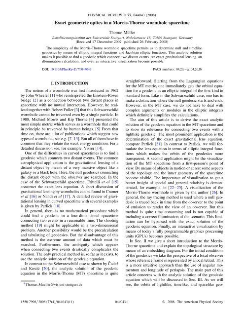
FIG. 1. Embedding diagram of the hypersurface h t
const;# =2 into the Euclidean space. The throat of the
wormhole is located at coordinate l 0. We will call the region
with l>0 the upper universe and the region with l

EXACT GEOMETRIC OPTICS IN A MORRIS-THORNE ... PHYSICAL REVIEW D 77, 044043 (2008)
L c 2 t_
2 l_
2 b 2 0 l 2 _’ 2 q
: (10)
k c 2 and h c b 2 0 l 2 i sin : (16)
From Eq. (8) there follow two constants of motion k, h with
c 2 t_
k and b 2 0 l 2 _’ h: (11)
B. Effective potential
The qualitative behavior of a geodesic can be studied
Inserting k and h into the Lagrangian (10) yields the
using the concept of an effective potential which is well
differential equation for the radial coordinate,
known from classical mechanics [29]. Equation (12) can be
l_
2 k 2 h 2
rewritten as an energy balance equation,
c 2 b 2 0 l 2 c 2 : (12)
l_
2 k 2
V eff
c 2 (17)
A. Initial conditions
with effective potential V eff c 2 h 2 = b 2 0 l 2
which is shown in Fig. 3. Because the effective potential
The initial conditions for the Eqs. (11) and (12) are given
depends mainly on h it can be interpreted as an angular
by the initial position t i ;l i ;’ i and the initial direction y
momentum barrier.
with respect to the local frame, Fig. 2.
Here, the initial direction y y t e t y l e l y ’ A geodesic rests on the same side of the wormhole
e ’ is
where it has started if V eff l 0 >k 2 =c 2 . In this case,
given by
the geodesic is deflected by the wormhole and reaches its
y y t closest approach l
e t cos e l sin e ’ (13a)
min . The point of reversal follows from
y t 1 the condition l_
0 and it is independent of the type of
c @ sin
t cos @ l q @ ’ (13b) geodesic,
b 2 0 l 2
t@ _ t l@ _
l
l _’@ ’ ; (13c)
2 h 2
min
k 2 =c 2 c 2 b 2 0 b 2 0 l 2 i sin 2 b 2 0 : (18)
where c for lightlike and c for timelike geodesics.
The velocity v=c is measured with respect to proaches the throat asymptotically. The corresponding
In the critical case V eff l 0 k 2 =c 2 the geodesic ap-
p
2
critical angle
the local frame and 1= 1 as usual. The time
crit is given by
direction y t follows from the local condition
b
crit arcsin 0
q : (19)
c 2 y t 2 y l 2 y ’ 2 : (14)
Thus, the time direction y t c for lightlike and y t
c for timelike geodesics. The sign depends on whether
the geodesic has to be traced back in time or should be
send to the future . The constants of motion k and h can
be expressed by these initial conditions. For lightlike geodesics
we have
q
k c 2 and h c b 2 0 l 2 i sin (15)
and for timelike geodesics the constants read
If V eff 0 and 0 . Note, that e l always points away
from the wormhole throat.
FIG. 3. Effective potential for a lightlike ( 0, k 2 =c 4 1)
and a timelike ( 1, k 2 =c 4 2 ) geodesic with initial
conditions: l i =b 0 6:0, 0:3, 0:6.
044043-3

THOMAS MÜLLER PHYSICAL REVIEW D 77, 044043 (2008)
geodesics at great length. So it becomes obvious that one
should represent the elliptic integrals by elliptic integral
functions.
1. Radial geodesics
For radial geodesics the Lagrangian (10) simplifies to
L
c 2 t_
2
_ l 2 : (20)
From the Euler-Lagrangian equations (8) together with the
initial conditions (15) and (16) we can immediately determine
the radial geodesics. Thus, from dl=dt
p
c 2 c 2 k 2 =c 2 =k 2 we obtain
l ct l i for 0; (21a)
l vt l i for 1: (21b)
Hence, an object with zero initial velocity, v
and rests at the initial radial position l i .
0, is static
2. Circular geodesics
From the effective potential, Fig. 3, we immediately see
that circular orbits only exist for l 0 and they are unstable.
Here, with l_
0, the Lagrangian reads
L
c 2 _ t 2 b 2 0 _’2 c 2 (22)
and the orbit ’ ’ t follows from d’=dt c 2 h= b 2 0 k ,
ct
’ ’
b i for 0; (23a)
0
’ vt ’
b i for 1: (23b)
0
Again, an object with zero initial velocity stays at the
initial angular position ’ i .
3. Arbitrary geodesics
In the case of arbitrary geodesics we consider the orbital
motion l l ’ . For that, we have to solve the differential
equation
dl 2 l_
2 c 2 k 2 =c 2
d’ _’ 2 h 2 b 2 0 l 2 2 b 2 0 l 2 (24)
which follows from Eq. (12). Transforming to the radial
q
coordinate r b 2 0 l 2 leads to the representation
dr 2
r 2 b 2 c 2 k 2 =c 2
0
d’
h 2 r 2 1 : (25)
Note that we have chosen only the positive sign for the
coordinate r. In order to still cover the whole spacetime, we
need two charts. The first chart represents the region l 0
and the other one represents l 0 and the initial angle lies
in the interval 0; for nonradial geodesics, we have a>
0. With the critical angle crit from (19) it follows:
8
< 1 for < crit or > crit
Thus, because r, b 0 , and a are strictly positive, is also
strictly positive. On the other hand, from the balance
equation (17) together with the condition l_
2 0 follows
that 1. In the following we will also use the scaled
q
distance b b 0 = b 2 0 l 2 instead of the parameter .
Note that Eq. (27) is independent of . Hence, all geodesics
follow the same orbit regardless of whether they are
timelike, lightlike, or spacelike. As can be easily shown,
this is also true for any spherically symmetric and static
spacetime.
Case 1: Ifa 0, negative sign). Note
that the root in Eq. (29) vanishes for l 0 and l l min .
However, the integral remains finite and we only have to
split it into two branches. For =2 l f l i we obtain
’
F i F ; a : (32)
On the other hand, if > =2, there is only a solution for
l f l min . In the case l f >l i , the angle ’ is given uniquely
by
’
2K a F ; a F i ; (33)
044043-4

EXACT GEOMETRIC OPTICS IN A MORRIS-THORNE ... PHYSICAL REVIEW D 77, 044043 (2008)
while if l f =2, l f l i . The orbital equation
’ reads
and thus,
crit
sinh’ cosh’ 1 b 2 i b i
cosh 2 ’ b 2 i sinh2 ’
s
1
l crit
b 0
1
2
crit
(51)
: (52)
In that case, a geodesic either starts with the critical angle
crit (lower sign) and recedes to infinity or it starts
with
crit and approaches the throat asymptotically
(upper sign). For
crit the angle ’ might
grow unlimited, while for crit the maximum angle
’ ? max reads
’ ? 1
max
2 ln1 b i
arsinh b 0
(53)
1 b i l i
which follows immediately from Eq. (50) with 0.
In Fig. 4 we collocated the function ’ ’ b , where
q
b b 0 = b 2 0 l 2 is the scaled distance, for all three above
044043-5

THOMAS MÜLLER PHYSICAL REVIEW D 77, 044043 (2008)
initial angle > =2 and ’ f >’ min is given by
l 2L 1 L i L f (58)
with f ’ f and i sin , whereas otherwise
l L f L i : (59)
If a>1, the primitive of Eq. (56) reads
R
L b 0 F a ; D a ; : (60)
FIG. 4. The angle
q
’ (ordinate) is plotted over the scaled
distance b b 0 = b 2 0 l 2 (abscissa), l 0. The throat size is
b 0 2 and the observer is located at l i 6 b i 0:316 . The
dotted line separates the destination points l f _ l i and the solid
line separates the initial angle _ =2. The dash-dotted line for
7
9
is composed of ’
b’ min and ’
’<
’ min .
mentioned cases. Because b does not distinguish between
the upper and lower universe, we restricted to l 0.
4. Length of a geodesic
The spatial length l of a geodesic follows from the
integral over the orbital curve C fl ’ ;’ 0...’ f g,
Z
l d~s; (54)
where d~s 2 dl 2 b 2 0 l 2 d’ 2 . If we use ’ as the orbital
parameter, the integral reads
s
Z dl 2
l
b 2 0 l 2 d’: (55)
C d’
Instead of the angle ’ we can also parametrize C by ,
Z
b
l
0
p d : (56)
C a 2 1
2
1 a 2 2
For a crit, we must distinguish
whether we measure the length up to the wormhole throat,
’ f

EXACT GEOMETRIC OPTICS IN A MORRIS-THORNE ... PHYSICAL REVIEW D 77, 044043 (2008)
the time t are shown in Fig. 6. Note that the angle cone is
limited to the interval 0; =2 . Measuring cone and t,we
can immediately read the throat size b 0 from Fig. 6.
Now, the distance of the observer to the wormhole throat
follows from Eq. (26),
p
b
l 0 1 a 2 conesin 2 cone
i : (66)
a cone sin cone
The scaled distance b i is given by b i a cone sin cone and is
shown in Fig. 7.
FIG. 6. The observation angle cone is plotted on the abscissa.
Left axis: The solid line represents the size of the throat b 0
scaled by the time t between the emission of the flash and the
observation of the ring. Right axis: The dashed line corresponds
to the parameter a cone .
the flash and the lightning up of the ring deciphers the size
of the throat. From c t l together with Eq. (58) we
obtain
1 c ta
b cone
0
2 A
where the denominator A is given by
(65)
A D a cone D sin cone ;a cone
q
cot cone 1 a 2 conesin 2 cone:
The parameter a cone as well as the throat size b 0 scaled by
V. CONNECTING TWO POINTS WITH A
LIGHTLIKE GEODESIC
Consider any two fixed points P and Q. Because of the
spherical symmetry and staticity of the MT metric, one can
always orientate a coordinate system such that P and Q
will lie in the hypersurface # =2 with P lying on the
x-axis, compare Fig. 8.
Without loss of generality we can choose the coordinates
of P and Q to be
P: l l i > 0; ’ 0;
Q: l l f ; ’ ’ f > 0:
To find the initial angle >0 of the geodesic which
connects P and Q in the Morris-Thorne spacetime with
fixed throat size b 0 , we have to solve the conditional
equation
C li ;l f ;’ f
’ l i ; ’ f
!
0; (67)
where ’ l i ; follows from ’
or ’
, respectively, and
the parameters l i , l f , and ’ f are fixed. Because of the
ambiguity of the Jacobian functions, we solve Eq. (67)
FIG. 7. The scaled distance b i is plotted with respect to the
observation angle cone. The proper distance l i is connected to
q
the scaled distance by l i b 0 bi 2 1. In the limit cone
=2, the observer is located in the throat.
FIG. 8. In MT spacetime a coordinate system can always be
chosen in such a way that any two points P and Q will lie in the
# =2 plane. A geodesic connecting both points has an initial
angle with respect to the direction of the wormhole throat.
Since there are arbitrary many geodesics connecting both points,
the angle is not unique. However, we can eliminate the
ambiguity of by fixing the angle ’ f .
044043-7

THOMAS MÜLLER PHYSICAL REVIEW D 77, 044043 (2008)
for the parameter a in the first place and then calculate ,
compare Eq. (26).
The most simple case is when P and Q lie in opposite
universes, l f < 0. Then, the geodesic connecting both
points has to pass the wormhole throat at ’ ’ throat b i ,
compare Eq. (47). Thus, the conditional Eq. (67) is composed
of ’ throat b f and ’ throat b i ,
C ? ’ throat b i ’ throat b f ’ f
and the initial angle
2 K F b i ; F b f ; ’ f ;
(68)
reads
arcsin b i : (69)
However, if l f 0, we have to determine the domain
where Q is localized in order to choose the correct orbital
equation ’ ’ ; a from Sec. III C 3. Therefore, we
have to plot the critical curves l crit
and l =2 for a given
initial position l i . Like in Fig. 4, we can use the scaled
q
coordinate b b 0 = b 2 0 l 2 instead of the proper coordinate
l, since l f 0, compare Fig. 9.
The separators b crit
follow from Eq. (52) where b crit
is
only valid in the range ’ 2 0;’ ? max . On the other hand,
the separator b =2 follows from Eq. (39) and is valid in the
range ’ 2 0; K =2 . While the geodesics in the regions
1 , 3 , and 4 are strictly monotonic, a geodesic in region 2
might have a place of closest approach b min depending on
the initial angle , compare Eqs. (18) and (35).
Now, we can determine the conditional equation C 0
for the different regions. If Q is located in region 1 or 4 ,
the conditional equation is simply given by
C 1 ;4 F b f ; sign b f b i
’ f
F b i ; ;
(70)
where 2 0; 1 . follows from arcsin b i a for Q 2
4 or arcsin b i a for Q 2 1 , respectively. If Q is
located in region 3 , we get the equation
C 3 a ’
a ’ f (71)
and the parameter a can be uniquely found in the range
b i ; 1 . The most complicated condition arises for Q 2 2 .
As long as l f >l i , the condition is given by
C 2
a ’
a ’ f : (72)
But, if l f ~’ min
compare Eqs. (33) and (34), respectively. The ambiguity
between and a is solved by comparing l f to the separating
curve l =2 . Thus, if ’ f < K a =2 and l f >l =2 ’ f
the initial angle is arcsin b i =a and
arcsin b i =a otherwise.
FIG. 9. The MT spacetime is divided into four regions which
are separated by the lines b crit
, b crit
and b =2 . Here, the angle ’ is
shown as a function of the scaled distance b for a wormhole with
throat size b 0 2 and an observer who is located at l i 6.
Geodesics with initial angle =2 < < crit have a point of
closest approach at b min , compare Eq. (18).
VI. GRAVITATIONAL LENSING
A review of gravitational lensing from a spacetime
perspective with a detailed list of references is given by
Perlick [18]. In general, gravitational lensing is only investigated
in the weak or strong field limit. Here, we follow
Perlick [21] and determine the exact lensing equation
L ; ’ 0 for the MT metric with parameters ’ and
as shown in Fig. 10. Because of the spherical symmetry of
the MT spacetime, we can restrict us to the # =2
plane. Note that, unlike Perlick, we evaluate the arising
elliptic integrals and determine the gravitational lensing
equation as well as the angular diameter distances by
means of elliptic integral functions.
As in the previous section, we have to connect two
points by a lightlike geodesic for the lensing equation.
044043-8

EXACT GEOMETRIC OPTICS IN A MORRIS-THORNE ... PHYSICAL REVIEW D 77, 044043 (2008)
FIG. 10. An observer located at position l i > 0 receives light
from a source at position l f ;’ at an angle .
While the observer is fixed at position l i , the position of the
light source is given by the fixed radius l f and an arbitrary
angle ’. However, in contrast to the previous section, we
do not solve the lensing equation for the initial angle but
for the position angle ’.
Depending on the position l f , we have to consider three
cases. The most simple one is given by l f < 0. For each
observation angle represented by sin =b i , we immediately
get the angle ’ of the source,
’ 2 K F b i ; F b f ; : (75)
Since the null geodesic must pass the wormhole throat, the
angle is limited to the range 1; 1 with 1
arcsin b i crit , compare Fig. 11.
If 0 l f crit there are two intersections
arcsin b i
b f
: (76)
’ 1 F f ;a F sin ; a ; (77a)
’ 2 2K a F f ;a F sin ; a ; (77b)
where the second one is hidden by the first one. On the
other hand, if min < < crit , the angle ’ is unambiguously
given by
’ F b f ; F b i ; ; (78)
compare Fig. 12. In the limiting case
min we obtain
’ min K b f F sin ; b f : (79)
In the third case, the position of the observer is closer to
the wormhole than the ring of sources, 0 l i l i .
To calculate image distortion and the brightness of
images one has to consider a congruence of null geodesics
starting at the observer’s position. For that, one has to
determine the radial and tangential angular diameter distances
D r ang and D t ang as described by Perlick [18]. For the
MT spacetime, we obtain
FIG. 11. Lensing ’ ’ for an observer located at l i 6
and rings with radius l f 0:1 (dashed line), l f 1 (solid
line), and l f 10 (dotted line).
FIG. 12. Lensing ’ ’ for an observer at l i 6 and rings
with radius l f 0:1 (solid line), l f 1 (dash-dotted line), l f
3 (dashed line). The dotted line marks the maximum angle
’ min for all l f , compare Eq. (79).
044043-9

THOMAS MÜLLER PHYSICAL REVIEW D 77, 044043 (2008)
observer
caustic
points
FIG. 13. Lensing ’ ’ for an observer at l i 6 and rings
with radius l f 7 (solid line), l f 10 (dotted line), l f 100
(dashed line).
q
D t ang b 2 0 l 2 sin’
f
(83)
sin
and
q
D r ang b 2 0 l 2 f
cos d’ (84)
d
with b i sin b f sin . As before, we have to identify the
necessary equations ’ ’ depending on the orbit of
the corresponding null geodesic. Instead of the angle ,we
can also calculate the derivative of ’ with respect to the
parameter a of Eq. (26) and then multiplying d’=da with
da
d
b 0 cos
q : (85)
sin 2 b 2 0 l 2 i
The derivatives of the elliptic integral functions F and K
are shown in the appendix.
VII. WAVE FRONTS
As in the previous sections, we use the geometric optics
approximation where light rays follow null geodesics in
curved spacetime. Then, a wave front at some coordinate
time t w const is defined by the corresponding endpoints
of all null geodesics starting from the initial event where
the flash of light was emitted. The conditional equation for
this wave front is given by
l ’;
!
W li
’;
t
c w 0: (86)
Here, only the position l i of the observer is fixed which is
also the point where the flash of light is emitted. For each
direction , we can calculate the length l of a geodesic by
means of the equations of Sec. III C 4. Figure 14 shows two
snapshots of a wave front which has started at time t 0.
FIG. 14. Embedding diagram of a wormhole with throat size
b 0 2. An observer located at position l i 10 emits a flash of
light at time t 0. The two solid lines represent the corresponding
wave front at time t w 4 and t w 16, respectively. At t w
16, the wave front overlap with itself resulting in two caustic
points.
The bending of light close to the wormhole throat lets the
wave front overlap with itself resulting in caustic points.
VIII. CONCLUDING REMARKS
Numerical libraries like, for example, the Numerical
Recipes [19] or the GNU Scientific Library [34] are able
to handle elliptic functions as well as Jacobian functions
like any other explicit function. Thus, there is no need to
numerically integrate the elliptic integrals. In the case of
gravitational lensing in the Morris-Thorne spacetime, compare
Sec. VI, we only have to evaluate the elliptic functions
at the initial and final points which speeds up the calculations.
In the more general case of connecting two arbitrary
points, we have obtained an easy to solve implicit
equation. Now, we are able to find any null geodesic which
connects an object with the observer or an arbitrary light
source. A physically reasonable illumination as well as an
interactive visualization becomes possible.
ACKNOWLEDGMENTS
This work was partly supported by the Deutsche
Forschungsgesellschaft (DFG), SFB 382, Teilprojekt D4.
APPENDIX: ELLIPTIC INTEGRALS AND
JACOBIAN FUNCTIONS
A detailed discussion of elliptic functions can be found
in Ref. [30]. Here, only a short collection of some relations
used in the main part of this article is given.
For the three basic Jacobian functions sn, cn, and dn, the
following identities hold
sn 2 u; k cn 2 u; k 1; (A1a)
dn 2 u; k k 2 sn 2 u; k 1; (A1b)
dn 2 u; k k 2 cn 2 u; k k 02 ; (A1c)
044043-10

EXACT GEOMETRIC OPTICS IN A MORRIS-THORNE ... PHYSICAL REVIEW D 77, 044043 (2008)
with k 02 k 2 1. If the module k of a Jacobian function the complete elliptic integral of the first kind is given by
vanishes, then we obtain the limiting functions
dK D
sn u; 0 sinu; cn u; 0 cosu; dn u; 0 1:
2
d 1 : (A5)
(A2)
At last, we need the derivatives of the elliptic integral of the
On the other hand, if k 1, the Jacobian functions simplify
to
that the argument as well as the module of the elliptic
first kind with respect to the parameter a or 1=a. Note
1
sn u; 1 tanhu; cn u; 1 dn u; 1
coshu :
integral depends on this parameter. Thus, we obtain
p
@F b; D b; F b; b 1 b
(A3)
2
p
@
2
1 2
1 1 2 b 2
If the module k 1, the incomplete elliptic integral of
the first kind, F , reduces to
(A6)
and
p
1 b 2
1
F u; 1 artanh u
2 ln1 x (A4)
1 x
while the elliptic integral of the second kind, D, simplifies
to D u; 1 u.
For the radial angular diameter distance D t ang, we need
the derivatives of the elliptic integrals. The derivative of
@F b a ;a
@a
D b a ;a F b a ;a
a 1 a 2 a
b
a
1
p
a 2 a 2 :
b 2
(A7)
[1] J. A. Wheeler, Geometrodynamics (Academic Press, New
York, 1962).
[2] A. Einstein and N. Rosen, Phys. Rev. 48, 73 (1935).
[3] R. W. Fuller and J. A. Wheeler, Phys. Rev. 128, 919
(1962).
[4] M. S. Morris and K. S. Thorne, Am. J. Phys. 56, 395
(1988).
[5] The metric presented by Morris and Thorne already appears
in 1973 by Homer G. Ellis [6]. However, he did not
recognize the metric as a wormhole but a drainhole.
[6] H. G. Ellis, J. Math. Phys. (N.Y.) 14, 104 (1973).
[7] M. Visser, Phys. Rev. D 39, 3182 (1989).
[8] E. Teo, Phys. Rev. D 58, 024014 (1998).
[9] M. Safonova, D. F. Torres, and G. E. Romero, Phys. Rev. D
65, 023001 (2001).
[10] M. Visser, S. Kar, and N. Dadhich, Phys. Rev. Lett. 90,
201102 (2003).
[11] P. K. F. Kuhfittig, Phys. Rev. D 68, 067502 (2003).
[12] A. DeBenedictis and A. Das, Classical Quantum Gravity
18, 1187 (2001).
[13] P. K. F. Kuhfittig, Phys. Rev. D 71, 104007 (2005).
[14] M. Visser, Lorentzian Wormholes—From Einstein to
Hawking (AIP Press, New York, 1995).
[15] S. Frittelli, T. P. Kling, and E. T. Newman, Phys. Rev. D
61, 064021 (2000).
[16] J. G. Cramer, R. L. Forward, M. S. Morris, M. Visser,
G. Benford, and G. A. Landis, Phys. Rev. D 51, 3117
(1995).
[17] K. K. Nandi, Y.-Z. Zhang, and A. V. Zakharov, Phys. Rev.
D 74, 024020 (2006).
[18] V. Perlick, Living Rev. Relativity 7, 9 (2004).
[19] W. H. Press, S. A. Teukolsky, W. T. Vetterling, and B. P.
Flannery, Numerical Recipes in C (Cambridge University
Press, Cambridge, England, 2002).
[20] A. Čadež and U. Kostić, Phys. Rev. D 72, 104024 (2005).
[21] V. Perlick, Phys. Rev. D 69, 064017 (2004).
[22] D. Weiskopf, Ph.D. thesis, Eberhard-Karls-Universität
Tübingen, 2001.
[23] D. Weiskopf, in Proceedings of the 16th IEEE
Visualization Conference, Minneapolis, 2005 (IEEE
Computer Society, New York, 2005).
[24] D. Weiskopf, IEEE Trans. Vis. Comput. Graph. 12, 522
(2006).
[25] U. Kraus, Eur. J. Phys. 29, 1 (2008).
[26] T. Müller, Am. J. Phys. 72, 1045 (2004).
[27] The metric (1) was firstly mentioned by Ellis [6] who
called it a drainhole. In contrast to Morris and Thorne he
identified the upper and lower universe.
[28] W. Rindler, Relativity—Special, General and Cosmology
(Oxford University Press, New York, 2001).
[29] H. Goldstein, Classical Mechanics (Addison-Wesley,
Reading, MA, 2002).
[30] D. F. Lawden, Elliptic Functions and Applications
(Springer-Verlag, New York, 1989).
[31] We use here the elliptic integral function F which is
related to the one given in Abramowitz and Stegun [32]
via F sin ; a F AS ; a .
[32] M. Abramowitz and I. A. Stegun, Handbook of
Mathematical Functions (Dover Publicaions, New York,
1964).
[33] R. P. Brent, Computer Journal 14, 422 (1971).
[34] GNU Scientific Library: http://www.gnu.org/software/gsl/.
044043-11