Car Side Window Kinematics - Institute of Geometry - Graz ...

Car Side Window Kinematics
A. Gfrerrer a , J. Lang a , A. Harrich b , M. Hirz b , J. Mayr b
a Institute of Geometry, Graz University of Technology, Austria
b Institute of Automotive Engineering, Graz University of Technology, Austria
Abstract
It is a demanding and time-consuming task to construct the side window
mechanism of a car such that the deflections along the seals are minimized.
The reason for this is that the window surface S delivered by the stylist, will
in general not be movable in a proper way: It is required that the surface
tightly moves along the seals. Deflections will necessarily occur no matter
how much effort the engineer invests. This article describes how to find
a spatial motion that minimizes seal deflection for some given automobile
side window surface. Necessary but acceptable modification of the stylist’s
surface S is also addressed, as well as the lifting mechanism design. It is
argued that our systematic approach offers considerable savings compared to
the prevailing trial-and-error approach.
Keywords:
space kinematics, car side window, window lifter mechanism
1. Introduction
Development of modern automotive products and systems is characterized
by accelerated production cycles, product diversification and quality
enhancement. Use of integrated virtual development methods that combine
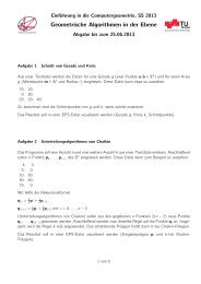
design, simulation and product management are continually sought. Fig.
1 shows the automotive door development process in the conceptual phase.
One major input is the car body styling. The styling data are transferred to
the computer aided engineering tools which, in turn, define a door concept
by iterative processes.
Email addresses: gfrerrer@tugraz.at (A. Gfrerrer), johann.lang@tugraz.at (J.
Lang), alexander.harrich@tugraz.at (A. Harrich), mario.hirz@tugraz.at (M. Hirz),
johannes.mayr@tugraz.at (J. Mayr)
Preprint submitted to CAD January 10, 2011

Styling
Door type
Ergonomics
& comfortf t
Door gap
s
t modules
Project
Turn in kinematics
Window kinematics
Se
ealing concept
Concept geometry
Package
Project duration
Structural
optimization
Figure 1: Exemplary automotive door development process in the conceptual phase
Boundary conditions defined by the car styling interact with various
engineering-based tasks. Ergonomic studies regarding the entrance area, the
seat position and door opening functionalities intimately interact with the
outer- (and later on with inner-) shape specifications of the door and its
neighboring components. The development of the door gap goes hand in
hand with a turn-in analysis and the hinge axis definition. Window kinematics
is a challenging door development problem.
Fig. 2 is a symbolic overview of the window kinematics layout process
including the main working packages and the data flow. The details of this
job are the main part of this paper.
Optimizing the layout of the window kinematics requires computations
not supported by commercially available CAD systems. Specific geometry
based data are exported into some CAD-external computation software. This
includes normals of a given window surface S as well as the B-pillar curve b,
the roof curve c and the daylight curve d (see Fig. 3).
The data are used to compute an optimized screw motion M of the given
window surface and an additional optimal window surface proposal S M . Window
lifter geometry is developed in a subsequent step. To this end two appropriate
anchor points Q, R are specified. The results are reimported to
2

CAD
• Styling surface
• Concept geometry
• Door packaging
Export of geometry
information (S, b, , c, d, Q, R)
Import of calculation
results (a, p,
S M , r)
CAD-external t lcalculation
l l • Screw motion M
• Surface proposal S M
• Lifter rail guide radius r
Figure 2: Car side window kinematics layout process
the CAD system and integrated into the conceptual door model to control
the corresponding geometries. Within the design process the window kinematics
can be evaluated in terms of its feasibility, packaging, function and
production.
Figure 3: A car side window S and its boundary curves d (daylight curve), b (boundary
curve towards the B-pillar) and c (roof curve).
In olden days cars had planar windows. Side windows moved vertically
and all points went in straight lines. Today, readily produced, curved car
windows contribute to strength, aesthetic and aerodynamic enhancement.
Of course a car window is basically a solid, bounded by a surface (exte-
3

ior boundary surface) and its offset surface (interior boundary surface) at
a certain distance (glass thickness). Additionally it is understood that the
window sheet is bounded all around. In the following we consider a surface
patch called S representing the exterior boundary of the window pane.
The geometry of a car side window is mainly driven by styling considerations.
The proposed window surface S is delivered by the stylist. It is the
engineer’s job to design an appropriate window lifting mechanism. The main
restriction is that the window has to be moved ‘in itself’. Implications of this
will be explained in Section 2. It is highly unlikely that a surface S delivered
by the stylist incidentally has this property. The engineer’s problem is virtually
unsolvable. However, small deflections, within limits, are acceptable. It
may be possible to find a motion which moves the surface S approximately
in itself.
Our approach follows the method suggested in [1], also applied in [2] and
[3]. In contrast to [1] we not only consider the given window surface S, but
also a curve b which eventually has to become a trajectory of the window
motion.
Our method delivers the screw motion M (or in special cases a revolution
or a translation) which best fits the given window surface S and the given
trajectory b (B-pillar, Section 4). The motion is determined by its screw axis
a and its pitch p. The value p in a screw motion is defined as the translatorial
distance per turn. With the optimal motion M in mind we can construct a
new window surface S M by subjecting the window roof curve to the motion
M. S M is a screw surface and perfectly moves in itself (Section 2). The given
surface S and the surface S M share the common roof curve. The maximum
distance between S and S M is a measure of the maximum deflection along
the seals of S (Section 6). This can be taken as a suitable ”figure of merit” of
the surface S that was proposed by the stylist. The motion M is the optimal
motion to be imposed on the given screw surface S and – at the same time
– to S M . M enables us to construct the optimal window lifter mechanism
(inside the door body, Section 7).
2. Moving Curves and Surfaces in Themselves
In this section we explain the concept of ‘movability in itself’ for curves
and surfaces. From a mathematical standpoint we deal with the invariant
curves and surfaces of one-parameter subgroups in the six-parameter Liegroup
SE(3) of Euclidean displacements.
4

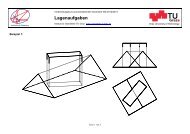
It is easy to understand that a straight line g can be moved in itself by a
parallel translation right in the direction of g. Such a motion moves any point
P on g into another point P ′ , again on the line g. The whole line remains the
same even if no single point on g keeps its position. Thus straight lines are
curves which can be moved in themselves. The same holds for circles where
the corresponding spatial motion is a revolution about the circle axis. Apart
from these two examples there is only one more type of curve to share this
property: the helix (Fig. 4). It can be moved in itself by subjecting it to the
corresponding screw motion.
Figure 4: Straight lines, circles and helices are the only curves which can be moved in
themselves.
This consideration, albeit theoretical, is applicable to the boundary curve
of a side window sheet, e.g. the one towards the B-pillar of a car. But we
also have to pose the same question for surfaces:
Which surfaces can be moved in themselves?
The answer is very similar to the answer in the curve case: There are three
types belonging to parallel translations, revolutions and screw motions. The
types are (Fig. 5)
• cylinder surfaces, generated by a curve being subjected to a parallel
translation.
• surfaces of revolution, generated by a curve subjected to a revolution
about an axis.
• screw surfaces, generated by a curve subjected to a screw motion.
5

Figure 5: Cylinders, surfaces of revolution and screw surfaces are the only surfaces which
can be moved in themselves.
In a way, the first two items can be viewed as special cases of the latter.
A rotation is a screw motion where the pitch vanishes, whereas a parallel
translation is the limit case of a screw motion where the pitch approaches
infinity. In these terms we can state:
Any window sheet moving in itself necessarily is a screw surface.
3. Preliminaries from Line Geometry
In the following we recall some well-known facts from line geometry which
we will need further on. For proofs and further details see [4, Chapter 3].
A straight line g in 3-space can be determined by its six ‘Plücker coordinates’
g 1 , g 2 , g 3 , g 1 , g 2 , g 3 .
These six numbers are usually collected in two 3-dimensional vectors
⎡ ⎤ ⎡ ⎤
g 1
g 1
g = ⎣ g 2
⎦ , g = ⎣ g 2
⎦ ,
g 3 g 3
called ‘normalized Plücker vectors’ of g. The term ‘normalized’ indicates that
the first Plücker vector g is of norm 1. The Plücker vectors of a line g can
be computed as follows: If g is a line with normalized direction vector d and
containing the point P whose position vector is p then
g = d,
g = p × d.
6

Due to this definition the Plücker vectors g, g of a straight line g have the
following properties:
• The components of g and g always satisfy the homogeneous quadratic
equation
Q : 〈g, g〉 = g 1 · g 1 + g 2 · g 2 + g 3 · g 3 = 0, (1)
called Plücker property. Here 〈., .〉 denotes the standard scalar product
of two vectors.
• Since g = d is a normalized direction vector of g we have
Q ∗ : 〈g, g〉 = g 2 1 + g 2 2 + g 2 3 = 1. (2)
• Replacing the point P ∈ g by another point Q ∈ g does not change the
second Plücker vector g of g.
By interpreting the Plücker coordinates g 1 , g 2 , g 3 , g 1 , g 2 , g 3 as coordinates
of a point G in the six-dimensional space R 6 we obtain a mapping
κ : g −→ G = κ(g)
from the set of oriented lines in 3-space to a set of points in R 6 (also compare
with [3]). As the coordinates g 1 , g 2 , g 3 , g 1 , g 2 , g 3 have to satisfy (1) and (2)
the image points G lie in the intersection G of the two quadratic surfaces Q
and Q ∗ in R 6 determined by these two equations:
• Q in Eq. (1) is a quadratic cone whose vertex lies in the coordinate
system origin.
• Q ∗ in Eq. (2) is a quadratic cylinder with 3-dimensional generator
spaces.
The four-dimensional intersection manifold G = Q∩Q ∗ is algebraic of degree
four.
Conversely, each point G ∈ G represents a uniquely determined oriented
line g in 3-space as follows:
Let g 1 , g 2 , g 3 , g 1 , g 2 , g 3 be the coordinates of G. After having put g :=
[g 1 , g 2 , g 3 ] ⊤ , g := [g 1 , g 2 , g 3 ] ⊤ the (normalized) direction vector of the line g
is
d = g,
7

whereas
p = g × g
is the position vector of a point P on g. By the way: P is the pedal point
on g w.r.t. the chosen origin.
As a conclusion we have that the mapping κ between the set of oriented
lines in 3-space and the set of points on the manifold G is a bijection.
Let now M denote a screw motion (or, as a special case, a pure rotation
or a pure translation). We consider the tangents of the paths generated by
M. They establish a vector field which can be written in the form:
ṗ = w × p + v
where v = [v 1 , v 2 , v 3 ] ⊤ , w = [w 1 , w 2 , w 3 ] ⊤ are constant vectors and ṗ denotes
the tangent vector of the point P with position vector p = [p 1 , p 2 , p 3 ] ⊤ (see,
for instance [5, p. 25]).
More precisely we have:
• M is a true screw motion if and only if w ≠ [0, 0, 0] ⊤ and 〈w, v〉 ≠ 0.
In this case
〈w, v〉
p = 2π
〈w, w〉
(3)
is the pitch of M,
d = w (4)
is a direction vector of the screw axis a and
a = w × v
〈w, w〉
(5)
is a position vector of a point A ∈ a.
• M is a rotation if and only if w ≠ [0, 0, 0] ⊤ but 〈w, v〉 = 0. Again the
axis of the rotation is determined just as in the screw motion case.
• The motion M is a translation (parallel to v) if and only if w =
[0, 0, 0] ⊤ .
8

Let g be a line orthogonal to the path c P (of a point P ) w.r.t. the motion
M. Then we obtain
0 = 〈ṗ, g〉 = 〈w × p + v, g〉 = det(w, p, g) + 〈v, g〉
= 〈w, p × g〉 + 〈v, g〉 = 〈w, g〉 + 〈v, g〉,
where g, g denote the Plücker vectors of g. Thus, the condition
〈v, g〉 + 〈w, g〉 = 0 (6)
characterizes the set of path normals of the motion M.
Eq. (6) is linear and homogeneous in the Plücker coordinates. Therefore,
interpreting this condition in the six-dimensional space R 6 , we have that the
point G = κ(g) lies in a hyperplane H O passing through the origin O.
The important conclusion is:
If we want to find a screw motion such that a given straight line g belongs
to its path normals, we have to look for a hyperplane H O of R 6 through the
origin containing the κ-image G = κ(g) of g.
Such a hyperplane in R 6 is determined by 5 points G 1 , . . . , G 5 in general
position (Fig. 6). Hence, in general we can find exactly one screw motion
(including the special cases mentioned above) to a set of five given lines
g 1 , . . . , g 5 as path normals.
Figure 6: The κ-images G i and hyperplane H O containing them.
Definition: The set of path normals of a screw motion M is called a
linear complex. It is denoted by L M .
4. Computing the optimal screw motion.
The method which we are following in this section has been suggested
in [1] and it has also been applied in [2] and [3]. If a surface S is moved in
9

itself, any point P ∈ S follows a path c P ⊂ S. This implies that the tangent
t P of c P is orthogonal to the surface normal n P . We are looking for some
screw motion M; so each surface normal n P is a path normal of M and thus
belongs to the line complex L M .
Let us return to the side window matter: In our case we have a set of
surface normals g i , i = 1, . . . n which are path normals to the screw motion
we are determined to find (Fig. 7, left). The κ-images G i = κ(g i ), i = 1, . . . n
of those normals form a ‘point cloud’ (Fig. 7, right). If we are given more
than five normals g (n > 5) under real-life conditions it is unlikely that the
corresponding point cloud lies exactly within one hyperplane H O through
the origin O. What we can try is finding a hyperplane through O which best
fits the point cloud, delivering the least square sum of deviations. This is the
core part of the calculation, an optimization process within the 6-dimensional
space R 6 . In the following we describe the single steps of this optimization
routine.
Figure 7: A set of surface normals {g i }, the corresponding κ-images {G i } in R 6 and the
optimal hyperplane H O .
Let g i , g i be the Plücker vectors of the line g i . If the points G i = κ(g i )
were indeed within a hyperplane we would have
〈v, g i 〉 + 〈w, g i 〉 = 0
for i = 1 . . . n with some coefficient vectors v, w. For our point cloud this
may not be the case.
10

If [v ⊤ , w ⊤ ] ⊤ = [v 1 , v 2 , v 3 , w 1 , w 2 , w 3 ] ⊤ denotes the normalized normal vector
of the yet unknown hyperplane H O , then the squared distance of the
point G i to H O is computed via
Hence, we have to minimize the sum
d 2 i = (〈v, g i 〉 + 〈w, g i 〉) 2 .
f(v, w) =
n∑
d 2 i (7)
i=1
of squared distances subject to the constraint
g(v, w) = v 2 1 + v 2 2 + v 2 3 + w 2 1 + w 2 2 + w 2 3 − 1 = 0. (8)
The constraint equation guarantees that the normal vector of H O has indeed
length 1.
Using a Lagrangian multiplier λ for this constraint leads to determining
the smallest eigenvalue of a positive semidefinite 6×6-matrix. For the details
the reader is referred to section 2 of [3].
The outcome of the optimization process is called M. In geometrical
terms M is a hyperplane through the origin O in the 6-space
M . . . 〈v, g i 〉 + 〈w, g i 〉 = 0.
In mathematical terms we have a 6-vector [v ⊤ , w ⊤ ] ⊤ = [v 1 , v 2 , v 3 , w 1 , w 2 , w 3 ] ⊤ .
5. A prescribed path
The method of [1] will now be modified by additionally considering a
given input curve. The motion M we found may be the best possible motion
for the given window surface. However, a side window sheet requires one
more thing: There is the boundary curve b towards the B-pillar, which is
prescribed. It is usually shaped as a seal slit and has to be a path of the
window motion M. We obtain additional constraints for the screw motion
M to be found.
If each normal to b belongs to the linear complex L M we can be sure that
b is moved in itself. This implies that b is a path of M, i.e., a helix.
If we are given the boundary curve b it – most probably – is not a helix.
We have to find a screw motion with a helical path as close to b as possible.
More precisely:
11

This screw motion M has to fit the window surface S and the B-pillar b
at the same time.
The fact that the surface normal in a point Q ∈ S belongs to the linear
complex L M signifies the condition that the path of Q is tangent to S in Q.
If Q belongs to the curve b we demand even more: The path tangent t Q to
Q is meant to be tangent not only to the window surface S but even to the
curve b ⊂ S. All the path normals to b in Q have to belong to the linear
complex L M . These path normals form a pencil of straight lines (Fig. 8).
Figure 8: The B-pillar b and its normals.
It is sufficient to pick two lines out of this pencil of lines. Each of these two
lines yields a condition which is of the same type as all the other conditions
for the surface normals n P of our window. We can add the surface normal
n Q in Q and one more line. The latter could be the line n ∗ Q with the direction
orthogonal to both t Q and n Q .
If we want to express that our motion M ought to have a trajectory ‘close
to the curve b’ we have to consider several points Q ∈ b and we have to add
a pair of lines for each of them. This adds up to a number of additional lines
which have to belong to the linear complex L M just as the surface normals.
We have a set of further conditions for our optimization problem. The task
itself, however, is of the same nature and the algorithm can basically remain
unchanged.
Remark: In real life examples we chose 100 surface normals for the window
sheet and 50 points along the curve b. Those 50 points Q delivered 50 surface
normals n Q and another 50 lines n ∗ Q . So we eventually had 200 straight lines
12

as the input for our optimization job. The lines yielded 200 points in the
5-space and our method delivered a hyperplane to this point cloud. This
hyperplane in turn symbolized a screw motion M.
We have achieved a window motion which fits the B-pillar in terms of
moving it in itself and, at the same time, fits the window sheet as perfectly
as possible.
Admittedly, there is still the question: How good is ‘as perfect as possible’?
This question is addressed in the next section.
6. Evaluating the surface
In the past the process of setting up a proper kinematic layout for a side
window pane has always been a delicate job. Whatever kinematic solution the
engineer brought forward, it was difficult to tell whether the flaws showing
up were due to the kinematic mechanism or already inherent in the given
window surface design. It is imperative to evaluate the result. To this end
we have to find some figure of merit for the outcome.
The screw motion M which we have found moves any screw surface (corresponding
to M) perfectly in itself. One such surface which is probably
pretty close to the given window sheet, could be constructed in the following
way:
We choose a curve c on the given window surface S. This might be any
curve e.g., the daylight curve of the window. However, we suggest taking the
border curve of S towards the roof together with the border curve towards
the A-pillar. We call this joint curve c the ‘roof curve’. If we subject this
curve c to the optimal screw motion M we create a screw surface S M .
The surface S M has the following properties
• S M moves in itself if the motion M is applied. There is no deflection
whatsoever.
• S M and S share the common roof curve c.
Let m be the maximum distance between S and S M . This value m is a
reliable measure for the maximum deflection caused by the screw motion M
if applied to the given window surface S.
The value m can be compared with the deflection limits of the seals
manufacturer. This way it is easy to tell whether the kinematic design is
within the design target. Just in case that the deflection value m exceeds
13

the limits, we have a good argument for returning the window sheet design
to the stylist. We can even add a suggestion for a perfect replacement S M
with the following appealing properties:
• S M differs from S by a margin which nowhere exceeds the value m.
• S M has the same roof curve c as the original proposal S.
• S M moves perfectly in itself.
If the method is applied at an early stage of the design process this may
lead to a perfect solution in the first place.
Remark: For experimental validation we applied the method to an example
which is already being produced, and which has already been tried and
tested. We arrived at a value m being a fraction of a millimeter. Had our
method been applied in the first place it would have surely avoided a lot of
cut-and-try.
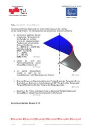
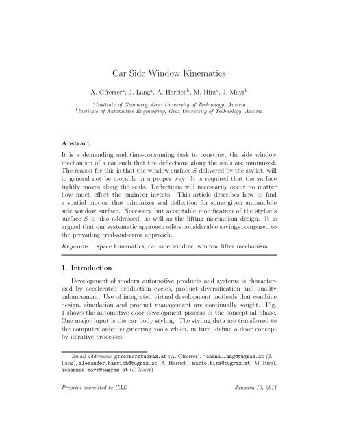
7. Constructing the lifter mechanism
Fig. 9 shows the configuration of a cable actuated window lifter mechanism
with two guides. This type of mechanism has a simple setup and is
commonly used in automotive front doors. The sliding blocks moving the
window glass are routed along the guide rails. The actuation is performed
by an electric motor (formerly by a hand crank) via a Bowden cable driving
the capstan.
Once we know the motion M it is easy to devise a suitable mechanism.
All we have to do is choose two appropriate anchor points and consider
their trajectories. These curves would, theoretically, be perfect guides (rails)
for the mechanism. We have to move each of the points on its respective
trajectory.
Of course there is always a difference between fundamental considerations
and real world applications with their real world constraints. We know the
window motion M is a screw motion with axis a and pitch p. A steady screw
motion moves every point in space with constant speed. Points with the
same speed lie on a right cylinder whose axis coincides with the screw axis a.
If there is only one lifter motor it is preferable choose anchor points moving
at the same speed to ensure that the lifter cable pulls equally at both rails.
As we know all the details about our screw motion M we can easily
see what this constraint brings about: We have to choose two points Q, R
14

cable connection
window surface
sliding block
sliding block
guide rail
guide rail
Figure 9: Cable actuated window lifter mechanism with two guides. The dark grey mechanical
component between the rails is the electric motor unit.
(anchor points, see Section 1) with equal distance from a. They must lie on
the same cylinder of revolution with the axis a. Of course the two points have
to be located near the bottom boundary curve of the window sheet. After
having selected one point the second can still be chosen on the corresponding
cylinder surface about a. We merely have to ensure there is no interference
within the door cavity.
Screw line rails are spatially curved. Rails in the form of a planar curve
are cheaper. The plane curve arc that most closely conforms to a helix is
circular. If we replace an optimal helix by an appropriate circle we certainly
have to accept some deviation from the ideal motion.
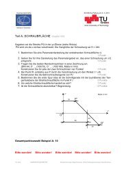
We can easily simulate the effect of replacing the helical rails by circular
ones. We choose 3 particular points P 1 , P 2 , P 3 on the helical arc and construct
a circle through these 3 points. Three suitable points are shown in Fig. 10,
(a).
In an actual design the helical and circular arcs conform much more
closely than those seen in Fig. 10, (a); to emphasize the distinction between
the two arcs we intentionally display the helical arc beyond its actually used
15

ange.
screw line arc
circular arc
Q
R
P 1
P 2 P 3
(a) Choosing 3 points P 1 , P 2 , P 3 on a helical arc
to find an appropriate circular approximation.
(b) Two appropriate anchor
points Q, R; their helical trajectories
are replaced by circular
arcs of equal radius.
Figure 10: Replacing the helical arcs by approximating circular segments.
Consider the following specific example with dimensions r (helix radius),
p (pitch) and h W (window height). The values r = 2000 mm, p = 600π mm
and h W = 400 mm deliver 1 a maximum difference between the helical arc
and the circular arc of less than 0.05 mm. The two circular rails have the
following properties:
• If the two anchor points Q, R (Fig. 10, (b)) are on the same cylinder of
revolution about the screw axis a, the two circular arcs have the same
radius.
• In this case the point paths along the two rails have the same length.
The motion M has the two points move with equal speed on their rails.
1 These figures are approximate but realistic.
16

• If the two anchor points are even on the same generator of the cylinder
of revolution about a and the two circular rails are parallel.
It is not necessary to locate the two anchor points on the same generator
(i.e., that they lie on a line parallel to the screw axis a). To have two rails
in parallel planes would not bring about any further benefits. It must be
pointed out here that the engineers’ concern that locating a pair of rails
in non-parallel planes would cause the mechanism to stall is unfounded. If
the engineer keeps this in mind he or she certainly has one more degree of
freedom in designing a lifter mechanism. Considering the confined space
within a door body, this may be important.
8. Conclusions
This article has treated the development of side window design from the
initially suggested stylist’s window surface all the way to the lifter mechanism.
The new method was characterized by the fact that we addressed the
problem from the bottom up. We worked with the most general set of spatial
motions which can move surfaces in themselves. The best motion for any
given window surface was derived. Further on we checked the given window
and evaluated its quality with respect to the force of friction exerted to the
seals. We then constructed a proper mechanism while providing a number
of free parameters such that the engineer could allow for spatial restrictions
that arise in the preparation of a suitable car door design.
An initial, poorly conceived window surface can be detected and then
modified only slightly so as to make it compatible with free movement as
well as the stylist’s original concept. There will be virtually no deflections
along the seals.
Hence, regardless of original window sheet suitability, there are two options.
No matter which way we go, we can easily use the optimal screw
motion M to construct a suitable window lifter mechanism. Replacing the
helical trajectories by circular ones reduces production cost.
In the development stage our approach will contribute considerable savings
– and quality improvement – in the development phase of the lengthy
and expensive process required to realize a new auto prototype.
The procedure was first outlined at SAE World Congress 2010 in Detroit,
USA [6]. Magna Steyr AG has successfully tested and applied our algorithm.
We have filed for a patent [7] at Deutsches Patentamt.
17

References
[1] H. Pottmann, T. Randrup, Rotational and Helical Surface Approximation
for Reverse Engineering, Computing 60, 1998, pp. 307–322.
[2] B. Odehnal, H. Stachel, The upper talocalcanean join, Technical Report
127, Geometry Preprint Series, Vienna Univ. of Technology, 2004, 12
pages, http://www.geometrie.tuwien.ac.at/odehnal/knochen.pdf
[3] H. Pottmann, M. Hofer, B. Odehnal, J. Wallner, Line Geometry for 3D
Shape Understanding and Reconstruction, in: T. Pajdla, J. Matas (Eds.),
Computer Vision – ECCV 2004, Part I, Vol. 3021 of Lecture Notes in
Computer Science, 1999, pp. 297–309.
[4] H. Pottmann, J. Wallner, Computational Line Geometry, Springer, 2000.
[5] O. Bottema, B. Roth, Theoretical Kinematics, Dover Publications, 1990.
[6] A. Harrich, J. Mayr, M. Hirz, P. Rossbacher, J. Lang, A. Gfrerrer, A.
Haselwanter, CAD-based synthesis of a window lifter mechanism, in: SAE
World Congress, 2010, Detroit, USA.
[7] A. Gfrerrer, J. Lang, M. Hirz, A. Harrich, J. Mayr, A. Haselwanter, G.
Bindar, Verfahren und Vorrichtung zum Ermitteln einer Sollbewegung,
zum Bewegen und zum Modifizieren eines verfahrbaren Bauteils, pat.
pend. DE10 2010 003 882.2, 12.04.2010, Deutsches Patentamt.
18

Authors biographies
Anton Gfrerrer received the M.S. degree in mathematics and descriptive
geometry from the University of Graz, Graz, Austria, in 1989 and the
Ph.D. degree from Graz University of Technology (TU Graz) in 1992. He is
currently an Associate Professor with the Institute for Geometry, TU Graz,
and also teaches at the University of Leoben. His research fields are geometry,
kinematics and robotics.
Johann Lang received his M.S. degree in mathematics and descriptive
geometry at Graz University in 1977 and his Ph.D. degree at Graz University
of Technology (TU Graz) in 1979. He is currently an Associate Professor with
the Institute for Geometry, TU Graz. His research fields are geometry and
kinematics.
Alexander Harrich was born 1982 in Klagenfurt, Austria.
Education: 2005 Master’s Degree in Automotive Engineering at University
of Applied Sciences FH Joanneum, Graz Job history: Since 2005 Scientific
researcher at Graz University of Technology, Institute of Automotive Engineering.
Research projects in the area of dynamic brake- and suspension
testing (2005 - 2008). Since 2008: Doctoral student at the Institute of Automotive
Engineering. Research field: Advanced design methods.
Mario Hirz was born 1973 in Austria.
Education: Master study of mechanical engineering and economic science at
Graz University of Technology. Doctoral study at the Institute of Internal
Combustion Engines and Thermodynamics.
Job history: Between 2000 and 2007: Vice head of the Section Design at the
Institute of Internal Combustion Engines and Thermodynamics. Since 2007:
Research assistant at the Institute of Automotive Engineering. Project manager
of several international engine- and vehicle research projects. Lecturer
at Universities and in the automotive industry in Europe and Asia. Research
activities in the area of virtual product development. About 90 publications,
several national and international awards.
Johannes Mayr was born 1984 in Graz, Austria.
Education: Study of Mechanical Engineering and Economics, Graz University
of Technology
Job history: From 2005 to 2008 design engineer in the automotive industry
at Magna Engineering Center. International experience in projects in Great
Britain and Saudi Arabia. Since 2008 research assistant at the Institute of
Automotive Engineering at Graz University of Technology. Research activities
in the area of 3D-CAD and development methods.
19