ipcc_defeat

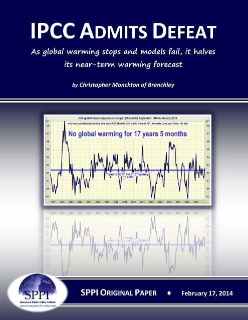
IPCC ADMITS DEFEAT
As global warming stops and models fail, it halves
its near-term warming forecast
by Christopher Monckton of Brenchley
SPPI ORIGINAL PAPER ♦ February 17, 2014

IPCC ADMITS DEFEAT
As global warming stops and models fail, it halves
its near-term warming forecast
by Christopher Monckton of Brenchley | February 17, 2014
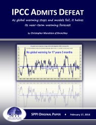
All you need to know about “global warming” is in this one simple graph. For 17 years 5
months, there has not been any global warming at all.
None of the computer models so imprudently relied upon by the Intergovernmental Panel on
Climate Change predicted that.
According to Remote Sensing Systems, Inc., the longest continuous period without any global
warming since the satellite record began in January 1979 is 17 years 5 months, or 209
successive months, from September 1996 to January 2014 inclusive.
Indeed, on the RSS dataset there has been no statistically-significant warming at 95%
confidence for almost a quarter of a century.
The Central England Temperature Record, the world’s oldest, which tracks global temperature
change well, shows no warming – at all – for 25 full calendar years.
2

The Central England Temperature Record, unlike the global record, shows a strong seasonal
signal from the summer peak to the winter trough each year.
The fastest supra-decadal rate of warming observed in any temperature record was recorded in
Central England from January 1694 to December 1733. During that 40-year period, temperature
in Central England, and probably worldwide as well, rose at a rate equivalent to 4.33 C° per
century.
Looking at the graph, it is evident that even this rapid warming rate represents only a small
fraction of seasonal temperature variability.
3

The warming occurred chiefly because the Maunder Minimum, a 70-year period from 1645-
1715 during which there were very few sunspots, had come to an end and solar activity had
begun to recover.
During the whole of the 20 th century, the fastest supra-decadal rate of global warming was
from January 1974 to December 2006, a 33-year period, when global temperature rose at a rate
equivalent to just 2 C° per century.
But it is not only the long absence of global warming that is becoming significant. It is the
growing discrepancy between prediction (the orange zone in the graph below) and observation
(the bright blue trend-line).
4

The IPCC’s best-estimate prediction, in red, is trending upward at an unexciting rate equivalent
to 1.33 C° per century. Gone are the days of predicting 3 C° per century. The real-world trend,
however, is if anything very slightly downward.
The orange prediction zone is taken from the final draft of the IPCC’s Fifth Assessment Report,
published in 2013. The upper bound of that zone, at 2.33 C° per century, was the best-estimate
prediction in the pre-final draft of the report, but expert reviewers including me made it plain
to the IPCC that its reliance on the failed computer models was no longer scientifically credible.
As a result, it is now actually predicting less warming for the next 30 years than in the past 30
years.
The next two graphs show how dramatic was the reduction in the IPCC’s near-term global
warming prediction between the pre-final and final drafts of the 2013 Fifth Assessment Report.
The IPCC has reduced its best-estimate prediction for warming over the next 30 years from 0.7
C°, equivalent to 2.33 C° per century, to just 0.4 C°, equivalent to only 1.33 C° per century.
The green prediction zone is visibly at the lower end of the models’ predictions. For the first
time, the IPCC has abandoned its previous reliance on climate models.
5

The IPCC’s dramatic and humiliating – but scientifically necessary – reduction in its projections
of near-term warming was set in train by a warning given to the December 2012 Doha climate
conference by the temporary delegate from Burma that there had been no global warming for
16 years.
National delegations at first reacted angrily to this
intervention. However, several delegations asked the UN’s
climate panel whether my assertion that there had been no
global warming for 16 years had been accurate.
In Melbourne, Australia, in February 2013, Dr. Rajendra
Pachauri, the climate-science head of the IPCC, quietly
admitted there had been no global warming for 17 years,
and suggested that perhaps the skeptics should be given a
fairer hearing than they had been getting.
However, had it not been for a single newspaper, The
Australian, his remark would have gone altogether
unreported in the world’s news media, for it did not fit the
Party Line to which they had for so long subscribed.
Where did the models go wrong? After all, the greenhouse
effect is real and measurable, so we should have expected
some global warming over the past 17½ years.
One problem is that the models had greatly underestimated
the capacity of natural variability to override the relatively
weak warming signal from manmade CO 2 and other
greenhouse gases.
They ignore or inadequately parameterize many important
climate processes and undervalue the net cooling effect not
only of non-radiative transports, such as evaporation and
tropical afternoon convection, but also of recent climate
events, such as the:
Where did the models
go wrong? After all, the
greenhouse effect is real
and measurable, so we
should have expected
some global warming over
the past 17½ years.
One problem is that
the models had greatly
underestimated the
capacity of natural
variability to override the
relatively weak warming
signal from manmade
CO 2 and other
greenhouse gases.
‣ “Parasol effect” of growth in emerging nations’ unfiltered particulate aerosols;
‣ Decline in solar activity since 1960;
‣ Cooling effect of the recent double-dip la Niña;
‣ Recent fall in the ratio of el Niño to la Niña oscillations;
‣ El Niño temperature spike of 1998, which has the effect of artificially depressing linear
trends starting from 1995-1998;
‣ Restoration of global cloud cover after the naturally-occurring decline observed
between 1983 and 2001 (Pinker et al., 2005);
‣ Current 30-year “cooling” phase of the Pacific Decadal oscillation; and
6

‣ Natural variability that has given us many long periods without warming in the past 150
years.
There are also many widely-recognized uncertainties in the models’ representation of the
underlying mathematics. It is worth reviewing just some of these uncertainties.
Uncertainties in particulate aerosol forcings
A substantial source of uncertainty is in the forcings from anthropogenic particulate aerosols,
which inhibit incoming solar radiance by a parasol effect. If, as Murphy et al. (2009) suggest,
negative aerosol forcings are approximately equal to the positive CO 2 forcing, existing
particulate aerosol emissions have been sufficient to counteract the entire radiative forcing
from CO 2 . Assuming that aerosol emissions are substantial renders climate sensitivity high by
much reducing the aggregate forcing whose consequence is global warming.
However, given that aerosol emissions are variable and are not well mixed in the atmosphere,
their forcing cannot be reliably constrained. In the Far East and in Africa, particulate emissions
have increased, while in the West they have declined in response to environmental controls,
one of the earliest of which was the Clean Air Act 1956 in the United Kingdom.
Therefore, it is not at present possible to say whether there has been a net increase in
anthropogenic particulate pollution. Nor is it possible to determine whether the anthropogenic
particulates represent an appreciable fraction of total particulates.
Murphy et al. (2009) show the negative radiative forcing from particulate aerosols as
being of the same order of magnitude as the positive forcing from CO 2 .
7

Uncertainties in determining individual feedbacks f n
The greatest source of uncertainty in the determination of climate sensitivity arises from
temperature feedbacks – additional, internal forcings that arise purely because temperature
has changed directly as a result of an external forcing, and in consequence of that temperature
change. It is accordingly denominated in Watts per square meter per Kelvin of externally-forced
warming.
No temperature feedback can be measured empirically or derived theoretically. Nevertheless,
feedbacks exist. For instance, by the Clausius-Clapeyron relation, a warmer atmosphere can
carry more water vapor, the most significant greenhouse gas owing to its high concentration.
However, the relation does not mandate that a warmer atmosphere must carry more water
vapor: merely that it may.
Similarly, the IPCC finds the cloud feedback strongly positive, while Spencer & Braswell (2010,
2011) find it appreciably negative. Lindzen & Choi (2009, 2011), comparing variations in seasurface
temperature with variations in outgoing long-wave radiation, found short-term climate
sensitivity to be 0.7 K per CO2 doubling, implying net-negative temperature feedbacks, in
contrast to 11 models that all showed strongly net-positive feedbacks and thus high climate
sensitivity.
In 11 climate models, as sea-surface temperature (x axis) rises, outgoing long-wave
radiation (y axis) falls. However, observation from the ERBE and CERES satellites
(center panel) shows the opposite. Diagram based on Lindzen & Choi (2009).
8

Uncertainty in determining the water vapor feedback
Column water vapor (cm) in total (blue), showing no trend in the lower troposphere (green)
and a downtrend in the mid-troposphere (red). From Prof. Ole Humlum (2013).
In IPCC’s understanding, the most substantial of the temperature feedbacks is that from water
vapor, which on its own approximately doubles the direct CO 2 forcing via Clausius-Clapeyron
growth in column water vapor as the atmosphere warms. However, water vapor is not well
mixed, particularly at sub-grid scale, so that anomalies in column water vapor are difficult to
measure reliably. Not all of the datasets show column water vapor increasing.
Uncertainties in tropical mid-troposphere temperature change
Santer (2003), followed by IPCC (2007), holds that in the tropical mid-troposphere at a pressure
altitude 300 mb, through increased water vapor at that altitude, anthropogenic greenhouse-gas
forcings cause a warming 2-3 times faster than at the tropical surface. This tropical midtroposphere
“hot spot”, highly visible on altitude-latitude plots of temperature change, is said
to be a fingerprint of anthropogenic warming that would not occur if non-greenhouse forcings
had caused the warming.
However, the model-predicted tropical mid-troposphere hot spot is not observed. Either
tropical surface temperature is not being measured correctly or the anthropogenic influence is
small. If the latter, climate sensitivity must be below the IPCC’s interval of projections.
9

Models predict the existence of a tropical mid-troposphere hot spot (top, IPCC, 2007, citing
Santer (2003); above left, Lee et al., 2007; above right, Karl et al., 2006). However the hot
spot is not observed (below: Karl et al., 2006).
10

Christy (2013) compared the projections of 73 climate models (whose average is the red arrow)
with observed tropical mid-troposphere temperature change since 1979. Every single one of
the models had over-predicted the warming of the tropical upper air – many of them
extravagantly.
Singer (2011), after a thorough examination of the discrepancy between modeling and
prediction, concludes:
“… the claim … that observed and modeled trends are ‘consistent’ cannot be considered as valid.”
Uncertainties in the behavior and influence of clouds
IPCC acknowledges that clouds are a major source of uncertainty. The maximum supra-decadal
global warming rate since 1850, equivalent to 2 K century –1 , was observed during the 33 years
1974-2006 (HadCRUT4).
Most of the then warming occurred from 1983-2001, when a naturally-occurring transient
reduction in global cloud cover caused 2.9 W m –2 radiative forcing (Pinker et al., 2005) (Fig. 15,
and see Monckton of Brenchley, 2010, for a discussion).
The warming ceased late in 2001 when the cloud cover returned to normal. For comparison,
the entire anthropogenic forcing in the two and a half centuries 1750-2012 is estimated at 2.3
W m –2 (IPCC, 2013, Fig. SPM.4).
11

Globally-averaged +o.16 W m –2 yr –1 trend (2.9 W m –2 in total) in the short-wave solar surface
radiative flux anomaly, 1983-2001, after removal of the mean annual cycle, arising from a
naturally-occurring diminution in cloud cover. Source: Pinker et al. (2005, Fig. 1).
Uncertainties in determining the sensitivity parameter λ t
In the models, the evolution over time of the climate-sensitivity parameter λ t represents the
incremental influence of putatively net-positive temperature feedbacks that triples the 1.2 K
direct warming projected to occur in response to the radiative consequences of a doubling of
CO2 concentration. The transient and equilibrium values of λ t are subject to large theoretical as
well as empirical uncertainties. There is even evidence in the literature for a net-negative
feedback sum, and hence for climate sensitivity

A: Feedback-driven evolution of the climate sensitivity parameter λ t on an illustrative
curve fitted to λ 0 = 0.31 K W –1 m 2 , rising rapidly in the first several centuries via IPCC’s
implicit mid-range estimates λ 100 = 0.44 K W –1 m 2 and λ 200 = 0.50 K W –1 m 2 , to its midrange
equilibrium estimate λ ∞ = 0.88 K W –1 m 2 , attained after 1-3 millennia (Solomon et
al., 2009). B: A plausible alternative evolution of λ t , following an epidemic curve and
accordingly showing little increase above its Planck value for 500 years.
First, the IPCC’s implicit values for λ t suggest an initially rapid rise over the first few centuries
followed by a slower, asymptotic approach to the equilibrium value λ ∞ after several millennia
(Fig. 11A, and see Solomon et al., 2009, for a discussion). However, it is no less plausible to
imagine an epidemic-curve evolution of λ t (Fig. 11B), where feedbacks come very slowly into
operation, then accelerate, then slow asymptotically towards equilibrium, in which event λ t
may remain for several centuries at little more than its instantaneous value, and climate
sensitivity may be only 1 K.
The second major uncertainty is that, though the feedback amplification relation, eqn. (9),
derived from process engineering (Bode, 1945), has a physical meaning in electronic circuitry,
where the voltage transits from the positive to the negative rail as the loop gain crosses the
singularity at γ = 1 (Fig. 12), it has no physical meaning in the climate, where it requires a
damping term, missing from the models, whose presence would greatly reduce climate
sensitivity. There is no identifiable physical mechanism by which net-positive temperature
feedbacks can drive global temperature towards +∞ at γ = 0.9999 and then towards –∞ at γ =
1.0001. Indeed, temperatures below absolute zero are non-existent.
13

Climate sensitivity ΔT dbl at CO 2 doubling (y axis) against feedback loop gains γ = λ 0 f on the
interval [–1, 3] (x axis), where λ 0 is the Planck sensitivity parameter 0.31 K W –1 m 2 and f is
the sum in W m –2 K –1 of all unamplified temperature feedbacks. The interval of climate
sensitivities given in IPCC (2007) is shown as a red-bounded region; a more physically
realistic interval is bounded in green. In electronic circuitry, the singularity at γ = +1 has a
physical meaning: in the climate, it has none. Eqn. (9) thus requires a damping term that is
absent in the climate models.
Given climate sensitivity 3.26 [2.0, 4.5] K (red-bounded region in Fig. 12) the interval of loop
gains implicit in IPCC (2007) is 0.64 [0.42, 0.74], well above the maximum γ = 0.1 (i.e., it is to the
right of the vertical blue line in Fig. 12) adopted by process engineers designing electronic
circuits intended not to oscillate. The IPCC’s value for γ is too close to the singularity at γ = 1 for
stability. A less improbable interval for γ is [–0.5, 0.1], giving a climate sensitivity ΔT dbl = 1 K
(green-bounded region in fig. 12), and implying a feedback sum close to zero.
The temperature-feedback damping term missing from eqn. (9) has a physical justification in
the formidable temperature homeostasis of the climate over the past 420,000 years (Fig. 13).
Absolute global temperature has varied by as little as 1% (3 K) either side of the median
throughout the past four Ice Ages, suggesting that feedbacks are barely net-positive, so that the
loop gain in the climate object may be significantly below the IPCC’s 0.64. Climate sensitivity,
therefore, may be little greater than 1 K.
14

Global temperature reconstruction over the past 420,000 years derived from δ 18 O anomalies in air
trapped in ice strata at Vostok station, Antarctica. To render the anomalies global, the values of the
reconstructed anomalies (y axis) have been divided by the customary factor 2 to allow for polar
amplification. Diagram based on Petit et al. (1999). Note that all four previous interglacial warm
periods, at intervals of 80,000-125,000 years, were at least as warm as the current warm period.
Uncertainty arising from chaotic behavior in the climate object
Mathematically, the climate behaves as a chaotic object, so that reliable long-term prediction
of future climate states is not available by any method. There are three relevant characteristics
of a chaotic object: first, that though its evolution is deterministic it is not determinable unless
the initial conditions at some chosen moment t 0 are known to a precision that will forever be
unattainable in the climate (sub-grid-scale processes being notoriously inaccessible); secondly,
that its behaviour is complex; and thirdly, that bifurcations in its evolution are no more likely to
occur in response to a major perturbation in one or more of the initial conditions than in
response to a modest perturbation.
The mathematical theory of chaos was first propounded by Lorenz (1963), though he did not
himself use the term “chaos”. He wrote –
“When our results concerning the instability of non-periodic flow are applied to the
atmosphere, which is ostensibly non-periodic, they indicate that prediction of the
sufficiently distant future is impossible by any method, unless the present conditions are
known exactly. In view of the inevitable inaccuracy and incompleteness of weather
observations, precise, very-long-range weather forecasting would seem to be nonexistent.”
Climate is long-range weather. In Mark Twain’s words, “Climate is what you expect: weather is
what you get.”
15

Giorgi (2005) draws attention to the distinction between predictability problems of the first
kind (the initial-value problem of projecting future climate states when radical evolutionary
bifurcations in the chaotic climate object can arise in response even to minuscule perturbations
in the initial conditions, and yet we do not know what the initial conditions of the climate
object were before the onset of industrialization), and of the second kind (difficulties in
predicting the evolution of the statistical properties of the climate object), and concludes that
the climate-change prediction problem has components of both the first and the second kind,
which are deeply intertwined.
Climatic prediction, then, is both an initial-state and a boundary-value problem, whose degrees
of freedom are of a similar order of magnitude to the molecular density of air at room
temperature, an intractably large number. It is also a non-linearity problem.
A heuristic will illustrate the difficulty. Benoit Mandelbrot’s fractal, a chaotic object, is described
by the remarkably simple iterative quadratic recurrence equation
| c a complex number (2)
The simplicity of eqn. (2) stands in stark contrast to the complexity of the climate object. In eqn.
(2), let the real part a of the complex number c = a + bi fall on the x axis of the Argand plane,
and let the imaginary part bi fall on the y axis, so that the output will be displayed as an image.
At t 0 , let z = 0.
The Mandelbrot fractal is like the climate object in that it is chaotic and non-linear, but is unlike
the climate object in that it its initial conditions are specified to great precision, and the
processes governing its future evolution are entirely known.
There is no initial-state problem, for we may specify the initial value of c to any chosen
precision. However, with the climate object, there is a formidable and in practice refractory
initial-state problem.
Likewise, we know the process, eqn. (12) itself, by which the Mandelbrot fractal will evolve,
whereas our knowledge of the evolutionary processes of the climate is incomplete.
Let c 1 (the top left pixel) be 0.2500739507702906 + 0.0000010137903618 i, and let c ∞ (the
bottom right pixel) be 0.2500739507703702 + 0.0000010137903127 i. The color of each pixel in
the output image is determined by plugging that pixel’s value c n into eqn. (12) and counting the
iterations before |z| reaches infinity (or here, for convenience, a bailout value 1000).
Up to 250,000 iterations are executed to determine each pixel. The startlingly complex and
quite beautiful image that our heuristic equation generates under these initial conditions is
below.
16

Festooned Maltese Cross generated by eqn. (12) under the specified initial conditions.
The heuristic demonstrates the three relevant characteristics of a chaotic object. First, the
evolution of the object is critically dependent upon minuscule perturbations in the initial
conditions. Even a small variation in the interval on which c falls would generate a quite
different image, or no image at all.
Secondly, a chaotic object (even when, as here, it is generated by the simplest iterative
function) is highly complex. Indeed, with some justification the Mandelbrot fractal has been
described as “the most complex object in mathematics”. Yet it is generated by a function vastly
simpler than the complicated and refractory multivariate partial differential equations that
describe the climate.
Thirdly, a chaotic object may exhibit numerous bifurcations, vulgo “tipping points” The image,
where each color change is a bifurcation, shows many bifurcations even though the initial and
terminal values of the interval of which the image is the map are identical to 12-13 decimal
places. Bifurcations are no less likely to occur in a near-unperturbed object than in an object
that has been subjected to a major perturbation.
For these reasons, reliable, long-term numerical weather prediction is not available by any
method, and there is no reason to suppose even that there will be more bifurcations (in the
form of more numerous or more severe extreme-weather events, for instance) in a very much
warmer climate than in a climate that changes little and slowly. In short, in an object that
behaves chaotically, such as the climate, the unexpected is to be expected, but it cannot be
predicted to a sufficient resolution to allow reliable determination of the relative magnitudes of
the various natural and anthropogenic contributions to climatic change.
17

IPCC (2007, §14.2.2.2) recognizes this Lorenz constraint on predictability:
“In climate research and modeling, we should recognize that we are dealing with a
coupled non-linear chaotic system, and therefore that the long-term prediction of
future climate states is not possible.”
IPCC had until recently attempted to overcome the Lorenz constraint by averaging the outputs
of an ensemble of general-circulation models to derive probability-density functions and
comparing the results with observed trends.
However, Singer (2011) demonstrated that obtaining a consistent trend value from any
individual model requires a minimum of 400 run-years (e.g., 20 20-year runs or 4 100-year
runs), but that for reasons of time and expense most models are run only once or twice and for
short periods. He showed that error arose if outputs of single-run and multi-run models were
combined. Finally, he demonstrated that the reliability of the models does not necessarily
increase with the magnitude of the radiative forcing assumed over the period of the model run.
As for the applicability of probability density functions to climate prediction, this too is
questionable, in that any credible PDF demands more – not less – data and precision than are
necessary to arrive at a simple interval of projections of future warming. Since the data have
proven insufficient to allow reliable prediction of the latter, they are a fortiori insufficient for
credible construction of the former.
All previous IPCC reports have exaggerated the rate of future global warming, just as the Fifth
Assessment Report’s predictions are already proving to be exaggerations. Indeed, the IPCC itself
admitted its past over-predictions in a graph circulated to expert reviewers in the pre-final draft
of its 2013 Fifth Assessment Report:
18

The discrepancy between prediction and fact is still more striking when the range of predictions
from the IPCC’s 1990 First Assessment Report are compared with reality:
19

Conclusion
On the evidence here presented, it is evident that there has been no global warming for up to
25 years; that the IPCC has admitted there has been no global warming for 17 years; that the
satellite record confirms this; that the gap between the models’ prediction and observed reality
is widening; that the IPCC itself has realized this and
has reduced its near-term forecast of warming over the
coming 30 years from 0.7 C° to 0.4 C°; that the IPCC’s On the evidence here
models have greatly underestimated the cooling effect
of a combination of natural influences offsetting the presented, it is evident that
warming that might otherwise have been expected in
there has been no global
response to the growing concentration of CO 2 and
other greenhouse gases; that the models are unable to warming for up to 25 years.
constrain the numerous uncertainties in the underlying
mathematics of climate to within an interval narrow
enough to permit reliable climate prediction; and that, The IPCC’s models have
even if the models were not thus hindered by
unconstrainable uncertainties, the chaotic behavior of greatly underestimated the
the climate, viewed as a mathematical object, is such
cooling effect of a
as to render the reliable, very-long-term prediction of
future climate states altogether beyond our powers. combination of natural
How, then, will those who have made their careers by
presenting climate change as though it were a grave,
manmade crisis respond as temperatures – though
they may well be higher at the end of this century than
at the beginning – fail to rise either at anything like the
rate predicted or to anything like the absolute value
predicted?
influences offsetting the
warming that might
otherwise have been expected
in response to the growing
concentration of CO 2 and
There has been much intellectual dishonesty on the other greenhouse gases.
extremist side of the climate debate. Therefore, some
scientists in the hard-line camp may well be tempted to
press for immediate and savage cuts in CO 2 emissions, so that they can claim – quite falsely –
that the continuing failure of the planet to warm (for even they can see it will not warm by
much) is the result of the costly mitigation measures they had advocated, rather than what
would have happened anyway.
20