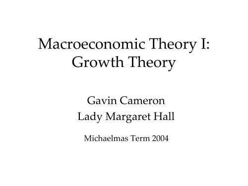
Macroeconomic Theory I: Growth Theory

Macroeconomic Theory I:
Growth Theory
Gavin Cameron
Lady Margaret Hall
Michaelmas Term 2004

macroeconomic theory course
• These lectures introduce macroeconomic models that have
microfoundations. This provides a neoclassical benchmark,
with optimising individuals and competitive markets. Of
course, incomplete markets and imperfect competition are
important phenomena in macroeconomics, but their effects are
perhaps best understood as deviations from a wellunderstood
benchmarks.
• In this lecture series we will examine:
• Growth Theory
• Investment
• Competitive Equilibrium (Real) Business Cycles
• New Keynesian Economics

the Ramsey model
• Ramsey (1928) analysed optimal economic growth under
certainty, by deriving the intertemporal conditions that are
satisfied on the optimal consumption path that would be
chosen by a central planner.
• Intertemporal optimisation is usually analysed by use of a
Hamiltonian function. This function maximises the present
value of utility over an infinite horizon with respect to a state
variable, a control variable, and a co-state variable (the shadow
price of an extra unit of the state variable in terms of utility).
This typically involves two first-order conditions and a
transversality condition (to ensure that the state variable
asymptotically approaches zero).

the OLG model
• Another approach to intertemporal optimisation is not to
assume that economic agents live forever, but to assume that
they live in overlapping generations, as pioneered by Allais
(1947), Samuelson (1958) and Diamond (1965).
• These models imply that at any one time individuals of different
generations are alive and trading with one another, and that
future generations may be neglected by current generations.
• The simplest possible such model, with just two generations alive
at any one time, is used extensively in life-cycle consumption
models.
• Chapter 2 of Romer (1996) provides a very good introduction
to both infinite-horizon and overlapping generations models.

a primer on growth theory
• In the Solow model, growth is exogenous since it is driven by
a rate of technical progress that is assumed to be constant.
• In the 1980s, economists became interested in models where
growth was endogenous, that is, was explained from within
the system.
• To do this, it is necessary to explicitly solve the consumer
optimisation problem of the economy - the Solow model omits
this by assuming a constant saving rate (although importantly
it does allow factor substitution).
• In practice, variables such as saving, human capital formation,
and R&D should be endogenous.

the development of growth theory
• Smith (1776), Malthus (1798), Ricardo (1817), Marx (1867)
• growth falls in the presence of a fixed factor
• Ramsey (1928), Cass (1965) and Koopmans (1965)
• growth with consumer optimisation (intertemporal substitution)
• Harrod (1939) and Domar (1946)
• models with little factor substitution and exogenous saving rate
• Solow (1956) and Swan (1956)
• factor substitution, an exogenous saving rate, diminishing
returns
• Arrow (1962) and Sheshinski (1967)
• growth as an unintended consequence of learning by doing

human capital models
• One-Sector Models
• with exogenous saving, diminishing returns: the Solow
model
• with exogenous saving and constant returns: the AK
model
• with consumer optimisation
• Two-Sector Models
• with exogenous saving: similar results to Solow model
• with consumer optimisation: the Rebelo model
• with consumer optimisation and no physical capital in
education: the Lucas-Uzawa model

human capital models
• What if production is not just a function of labour and capital,
but also depends upon human capital?
• Workers can be given the incentive to spend time learning
new skills if those skills will receive higher rewards in the
workplace.
• Therefore, we can have a perfectly competitive production
sector with human capital as an input into production.
• The simplest way to do this is to treat human capital as just
another form of capital (i.e. for it to be produced using the
same production function as physical capital and output): a
one-sector model.
• The harder way to do this is to treat human capital as being
produced by a different production function, presumably this
production function will itself be relatively intensive in
human capital: a two sector model.

a one-sector model (endogenous saving)
• Assume a standard Cobb-Douglas production function with human
capital input of H (i.e. the workforce L times the average quality of
the workforce, h):
(1)
1
Y AK α −α
= H = C+ IK
+ IH
• Changes in capital stocks are given by:
(2) K
= IK
−δK
H
= IH
−δH
• The equilibrium growth rate of C, Y, K and H can be shown to be
* α (1 −α)
(3) γ = (1/ θ).[A α .(1 −α) −δ−ρ]
• Where 1/θ is the inter-temporal elasticity of substitution of utility
and θ>0 (when θ is low, households care little about consumption
smoothing) and ρ is the rate of time preference.
• It should be apparent that there are constant returns to broad capital
in this model, and it consequently behaves like the AK model. All
variables grow at the rate of equation (3). Indeed, where
nonnegative gross investment is allowed, the model has no
transitional dynamics either since if K and H are unbalanced, they
adjust discretely to their equilibrium values.

a two-sector model (exogenous saving)
• Once again, consider the human-capital augmented model:
α 1−α
(4) Y=
K (hL)
• Where h is human capital per person. This evolves according
to:
(5) h = (1−u)h
• Where (1-u) is time spent learning and u is time spent working
. Re-writing this shows that an increase in time spent learning
raises the growth rate of human capital.
(6) h/h = (1−u)
• This models works just like the Solow model where we call A
human capital and let g=(1-u). Therefore, in this simple twosector
model, a policy that leads to a permanent increase in
the time spent learning leads to a permanent rise in the
growth of output per worker.

the Lucas-Uzawa model
• In the full Lucas-Uzawa model, the proportion of time spent
learning is endogenous. Consider the following output and
human capital accumulation equations:
α 1−α
Y= C+ K
+δ K = AK .(uH) H
+δ H= B.(1−
u)H
• To find the steady-state we look for a solution where u, K/H
and C/K are constant. In which case, the common growth
rate in steady-state of C, K, H, and Y is
*
(7) γ = (1/ θ)(B −δ−ρ)
• If we define the following
(8) ϕ≡[ ρ+δ.(1 −θ) ]/ Bθ
• Then the steady-state proportion of time devoted to not
learning is
(9)
*
u =ϕ+ ( θ−1)/
θ

dynamics of Lucas-Uzawa
• In general, the growth rate of consumption in the model is
(1 −α) −(1 −α)
(10) γ
C
= (1/ θ).[ αA.u ( ω) −δ−ρ]
• Where ω=K/H. Notice that (10) is inversely related to (K/H). Hence,
the growth rate tends to rise with the amount of the imbalance
between human and physical capital if human capital is abundant
relative to physical capital (ωω*).
• The model therefore predicts that the economy recovers faster from a
war that destroys physical capital than from an epidemic that
destroys human capital (the one-sector model predicts equally fast
recoveries from either).
• This is the result of the assumption that education is relatively
intensive in human capital. If ω>ω*, the marginal product of human
capital in the goods sector is high and so are wages. But the
education sector is relatively intensive in human capital and therefore
has a high cost of operation and low output.

ideas-based growth models
• Linear Knowledge Production Function
• Romer/Grossman-Helpman/Aghion-Howitt
• Non-linear Knowledge Production Function
• Jones/Kortum/Segerstrom
• Linear Increasing Variety
• Young/Peretto/Aghion-Howitt/Dinopolous-Thompson
• Non-Linear Increasing Variety
•Jones

the Romer model
• One of the most influential new growth models is that of Romer
(1990) which stresses the importance of profit-seeking research in the
growth process.
• There are three sectors in the full Romer model:
• A competitive production sector;
• A monopolistic intermediate-goods sector that produces
particular capital goods using designs purchased from the
research sector;
• A monopolistic research sector where inventors race to invent
and then receive a patent from the government.
• The aggregate production function exhibits increasing returns since
there are constant returns to L and K but ideas, A, are also an input.
• Increasing returns require imperfect competition. Firms in the
intermediate-goods sector are monopolists so capital goods sell for
more than their marginal cost.
• However, the profits of intermediate-goods firms are extracted by
inventors and compensate them for the time spent in inventing.
• There are no economic rents in the model; all rents compensate some
factor input.

the basic Romer model
• The aggregate production function takes the familiar form:
α
(11) Y=
K (AL )
Y
1−α
• There are constant returns to labour and capital but the
presence of ideas (A) leads to increasing returns overall.
Capital accumulates at the rate:
(12) K
= s Y−dK
K
• And the workforce grows at a constant rate:
(13) L/L = n
• Labour is used to either produce new ideas or to produce
output
(14) L + L = L
A
Y

ideas-based growth
• Views of the knowledge production function:
A
A = δ L
(15) R/GH/AH
A
(16) A
= δ LA φ
J/K/S
A
(17)
A
= δ LA
λ
A
φ
• δ is the productivity of each researcher; L A is the number of
researchers
• φ is the returns to the stock of ideas
φ>0 increasing returns to ideas ‘standing on shoulders’
φ

early endogenous growth
Romer/Grossman-Helpman/Aghion-Howitt
(18) Y = A σ
L Y There are constant returns to rivalrous inputs
and increasing returns to labour and ideas together, σ >0.
New ideas are produced using research labour and the
existing stock of knowledge:
(19) where L A
=sL and L Y
=(1-s)L with 0

semi-endogenous growth
Jones/Kortum/Segerstrom
A
= δ LA φ
(21)
A
Where φ>0 increasing returns to ideas and φ

growth with increasing variety
Young/Peretto/Aghion-Howitt/Dinopoulos-Thompson
Suppose that consumption is a constant-elasticity of substitution (CES) aggregate of a variety
of goods:
i i
(25)
0
where B is the number of different varieties of goods, Y i
is the consumption of variety i and
θ>1 is related to the elasticity of substitution between goods. The total number of varieties
evolves over time according to:
(26) B = L β
in Y/P/AH/DT models, β=1 so that the variety of goods is proportional to the population.
Under a range of assumptions about Y i
, per capita output is given by:
(27) c B A A
with the R/GH/AH knowledge production function, the growth rate of A depends on
research effect per variety, L A
/B:
(28) A
substituting this into equation (27) yields:
(29)
= ⎡ ⎤
⎢ ∫
⎣ ⎥ ⎦
B
1/ θ
C Y d
θ
g = θ g + σg = θβn + σg
1−
g = δ sL/
B=
δ sL β
1−
g = θβn+
σδsL β
c

the Jones (1999) model
The Y/P/AH/DT models assumed that β=1. The intuition for this is
that as the population grows, the number of varieties grows in
proportion so that the number of researchers per variety stays
constant. Therefore, there is no growth effect of scale.
If β1, there is a negative
growth effect of scale.
In addition, we can also look at the effect of the J/K/S knowledge
production function, A
= δ LA φ , on the growth rate of
A
output in (29):
(30)
L
1−β
g = θβ n+
σδ s
c
A
1−φ
This general models encompasses each of the three cases discussed
earlier.

the Jones model
β
φ=1
J/K/S
Y/P/AH/DT
Explosive or
J/K/S
β=1
J/K/S
Explosive
R/GH/AH
φ

optimal growth
• In human capital models, the investment rate chosen by the
representative agent is typically Pareto-optimal.
• In ideas-based models, the investment rate chosen by the
social planner is rather different from that chosen by the
market. This is due to four distortions:
• Current research affects the productivity of future research, but
this is not rewarded – standing on shoulders.
• Current research may also duplicate existing research and hence
lower the productivity of research – stepping on toes.
• Inventors cannot appropriate the entire consumer surplus due to
their inventions – surplus appropriability.
• Inventions may reduce the profitability of previous inventions –
creative destruction.

intuition and growth models
• To generate permanent growth in the absence of
population growth (a growth effect of scale), a
model must contain a fundamental linearity in a
differential equation.
• In the AK model this occurs in the production
function and in the Romer model this occurs in the
technology equation.
• In the Young-Peretto model this occurs in the
growth rate of varieties equation.
• The Lucas model of human capital also contains
such a linearity if u is assumed exogenous or when
there are constant returns to H and K.

you can download the pdf files from:
http://www.nuff.ox.ac.uk/Users/Cameron/lmh/