Reliable Fiducial Detection in Natural Scenes - University of Oxford
Reliable Fiducial Detection in Natural Scenes - University of Oxford
Reliable Fiducial Detection in Natural Scenes - University of Oxford

You also want an ePaper? Increase the reach of your titles
YUMPU automatically turns print PDFs into web optimized ePapers that Google loves.
<strong>Reliable</strong> <strong>Fiducial</strong> <strong>Detection</strong> <strong>in</strong> <strong>Natural</strong> <strong>Scenes</strong><br />
David Claus and Andrew W. Fitzgibbon<br />
Department <strong>of</strong> Eng<strong>in</strong>eer<strong>in</strong>g Science,<br />
<strong>University</strong> <strong>of</strong> <strong>Oxford</strong>, <strong>Oxford</strong> OX1 3BN<br />
{dclaus,awf}@robots.ox.ac.uk<br />
Abstract. <strong>Reliable</strong> detection <strong>of</strong> fiducial targets <strong>in</strong> real-world images is<br />
addressed <strong>in</strong> this paper. We show that even the best exist<strong>in</strong>g schemes are<br />
fragile when exposed to other than laboratory imag<strong>in</strong>g conditions, and<br />
<strong>in</strong>troduce an approach which delivers significant improvements <strong>in</strong> reliability<br />
at moderate computational cost. The key to these improvements<br />
is <strong>in</strong> the use <strong>of</strong> mach<strong>in</strong>e learn<strong>in</strong>g techniques, which have recently shown<br />
impressive results for the general object detection problem, for example<br />
<strong>in</strong> face detection. Although fiducial detection is an apparently simple<br />
special case, this paper shows why robustness to light<strong>in</strong>g, scale and foreshorten<strong>in</strong>g<br />
can be addressed with<strong>in</strong> the mach<strong>in</strong>e learn<strong>in</strong>g framework with<br />
greater reliability than previous, more ad-hoc, fiducial detection schemes.<br />
1 Introduction<br />
<strong>Fiducial</strong> detection is an important problem <strong>in</strong> real-world vision systems. The<br />
task <strong>of</strong> identify<strong>in</strong>g the position <strong>of</strong> a pre-def<strong>in</strong>ed target with<strong>in</strong> a scene is central<br />
to augmented reality and many image registration tasks. It requires fast, accurate<br />
registration <strong>of</strong> unique landmarks under widely vary<strong>in</strong>g scene and light<strong>in</strong>g<br />
conditions. Numerous systems have been proposed which deal with various aspects<br />
<strong>of</strong> this task, but a system with reliable performance on a variety <strong>of</strong> scenes<br />
has not yet been reported.<br />
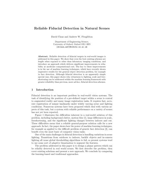
Figure 1 illustrates the difficulties <strong>in</strong>herent <strong>in</strong> a real-world solution <strong>of</strong> this<br />
problem, <strong>in</strong>clud<strong>in</strong>g background clutter, motion blur [1], large differences <strong>in</strong> scale,<br />
foreshorten<strong>in</strong>g, and the significant light<strong>in</strong>g changes between <strong>in</strong>doors and out.<br />
These difficulties mean that a reliable general-purpose solution calls for a new<br />
approach. In fact, the paper shows how the power <strong>of</strong> mach<strong>in</strong>e learn<strong>in</strong>g techniques,<br />
for example as applied to the difficult problem <strong>of</strong> generic face detection [2], can<br />
benefit even the most basic <strong>of</strong> computer vision tasks.<br />
One <strong>of</strong> the ma<strong>in</strong> challenges <strong>in</strong> fiducial detection is handl<strong>in</strong>g variations <strong>in</strong> scene<br />
light<strong>in</strong>g. Transitions from outdoors to <strong>in</strong>doors, backlit objects and <strong>in</strong>-camera<br />
light<strong>in</strong>g all cause global threshold<strong>in</strong>g algorithms to fail, so present systems tend<br />
to use some sort <strong>of</strong> adaptive b<strong>in</strong>arization to segment the features.<br />
The problem addressed <strong>in</strong> this paper is to design a planar pattern which can<br />
be reliably detected <strong>in</strong> real world scenes. We first describe the problem, then<br />
cover exist<strong>in</strong>g solutions and present a new approach. We conclude by compar<strong>in</strong>g<br />
the learn<strong>in</strong>g-based and traditional approaches.
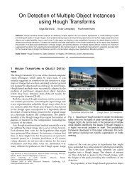
Church Lamp Lounge<br />
Bar Multiple Library<br />
Fig. 1. Sample frames from test sequences. The task is to reliably detect the targets<br />
(four disks on a white background) which are visible <strong>in</strong> each image. It is a claim <strong>of</strong> this<br />
paper that, despite the apparent simplicty <strong>of</strong> this task, no technique currently <strong>in</strong> use is<br />
robust over a large range <strong>of</strong> scales, light<strong>in</strong>g and scene clutter. In real-world sequences,<br />
it is sometimes difficult even for humans to identify the target. We wish to detect the<br />
target with high reliability <strong>in</strong> such images.<br />
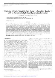
(a) (b) (c) (d) (e)<br />
Fig. 2. Overall algorithm to locate fiducials. (a) Input image, (b) output from the fast<br />
classifier stage, (c) output from the full classifier superimposed on the orig<strong>in</strong>al image.<br />
Every pixel has now been labelled as fiducial or non-fiducial. The size <strong>of</strong> the circles<br />
<strong>in</strong>dicates the scale at which that fiducial was detected. (d) The target verification step<br />
rejects non-target fiducials through photometric and geometric checks. (e) <strong>Fiducial</strong><br />
coord<strong>in</strong>ates computed to subpixel accuracy.
2 Previous work<br />
<strong>Detection</strong> <strong>of</strong> known po<strong>in</strong>ts with<strong>in</strong> an image can be broken down <strong>in</strong>to two phases:<br />
design <strong>of</strong> the fiducials, and the algorithm to detect them under scene variations.<br />
The many proposed fiducial designs <strong>in</strong>clude: active LEDs [3, 4]; black and white<br />
concentric circles [5]; coloured concentric circles [6, 7], one-dimensional l<strong>in</strong>e patterns<br />
[8]; squares conta<strong>in</strong><strong>in</strong>g either two-dimensional bar codes [9], more general<br />
characters [10] or a Discrete Cos<strong>in</strong>e Transform [11]; and circular r<strong>in</strong>g-codes [12,<br />
13]. The accuracy <strong>of</strong> us<strong>in</strong>g circular fiducials is discussed <strong>in</strong> [14]. Three dimensional<br />
fiducials whose images directly encode the pose <strong>of</strong> the viewer have been<br />
propsed by [15]. We have selected a circular fiducial as the centroid is easily and<br />
efficiently measured to sub-pixel accuracy. Four known po<strong>in</strong>ts are required to<br />
compute camera pose (a common use for fiducial detection) so we arrange four<br />
circles <strong>in</strong> a square pattern to form a target. The centre <strong>of</strong> the target may conta<strong>in</strong><br />
a barcode or other marker to allow different targets to be dist<strong>in</strong>guished.<br />
Naimark and Foxl<strong>in</strong> [13] identify non-uniform light<strong>in</strong>g conditions as a major<br />
obstacle to optical fiducial detection. They implement a modified form <strong>of</strong> homomorphic<br />
image process<strong>in</strong>g <strong>in</strong> order to handle the widely vary<strong>in</strong>g contrast found<br />
<strong>in</strong> real-world images. This system is effective <strong>in</strong> low-light, <strong>in</strong>-camera light<strong>in</strong>g, and<br />
also strong side-light<strong>in</strong>g. Once a set <strong>of</strong> four r<strong>in</strong>g-code fiducials have been located<br />
the system switches to track<strong>in</strong>g mode and only checks small w<strong>in</strong>dows around the<br />
known fiducials. The fiducial locations are predicted based on an <strong>in</strong>ertial motion<br />
tracker.<br />
TRIP [12] is a vision-only system that uses adaptive threshold<strong>in</strong>g [16] to<br />
b<strong>in</strong>arize the image, and then detects the concentric circle r<strong>in</strong>g-codes by ellipse<br />
fitt<strong>in</strong>g. Although the entire frame is scanned on start-up and at specified <strong>in</strong>tervals,<br />
an ellipse track<strong>in</strong>g algorithm is used on <strong>in</strong>termediate frames to achieve<br />
real-time performance. The target image can be detected 99% <strong>of</strong> the time up to<br />
a distance <strong>of</strong> 3 m and angle <strong>of</strong> 70 degrees from the target normal.<br />
CyberCode [9] is an optical object tagg<strong>in</strong>g system that uses two-dimensional<br />
bar codes to identify object. The bar codes are located by a second moments<br />
search for guide bars amongst the regions <strong>of</strong> an adaptively thresholded [16] image.<br />
The light<strong>in</strong>g needs to be carefully controlled and the fiducial must occupy a<br />
significant portion <strong>of</strong> the video frame.<br />
The AR Toolkit [10] conta<strong>in</strong>s a widely used fiducial detection system that<br />
tracks square borders surround<strong>in</strong>g unique characters. An <strong>in</strong>put frame is thresholded<br />
and then each square searched for a pre-def<strong>in</strong>ed identification pattern. The<br />
global threshold constra<strong>in</strong>s the allowable light<strong>in</strong>g conditions, and the operat<strong>in</strong>g<br />
range has been measured at 3 m for a 20×20 cm target [17].<br />
Cho and Neumann [7] employ multi-scale concentric circles to <strong>in</strong>crease their<br />
operat<strong>in</strong>g range. A set <strong>of</strong> 10 cm diameter coloured r<strong>in</strong>gs, arranged <strong>in</strong> a square<br />
target pattern similar to that used <strong>in</strong> this paper, can be detected up to 4.7 m<br />
from the camera.<br />
Motion blur causes pure vision track<strong>in</strong>g algorithms to fail as the fiducials are<br />
no longer visible. Our learnt classifier can accomodate some degree <strong>of</strong> motion<br />
blur through the <strong>in</strong>clusion <strong>of</strong> relevant tra<strong>in</strong><strong>in</strong>g data.
These exist<strong>in</strong>g systems all rely on transformations to produce <strong>in</strong>variance<br />
to some <strong>of</strong> the properties <strong>of</strong> real world scenes. However, light<strong>in</strong>g variation,<br />
scale changes and motion blur still affect performance. Rather than image preprocess<strong>in</strong>g,<br />
we deal with these effects through mach<strong>in</strong>e learn<strong>in</strong>g.<br />
2.1 <strong>Detection</strong> versus track<strong>in</strong>g<br />
In our system there is no prediction <strong>of</strong> the fiducial locations; the entire frame<br />
is processed every time. One way to <strong>in</strong>crease the speed <strong>of</strong> fiducial detection is<br />
to only search the region located <strong>in</strong> the previous frame. This assumes that the<br />
target will only move a small amount between frames and causes the probability<br />
<strong>of</strong> track<strong>in</strong>g subsequent frames to depend on success <strong>in</strong> the current frame. As a<br />
result, the probability <strong>of</strong> successfully track<strong>in</strong>g through to the end <strong>of</strong> a sequence is<br />
the product <strong>of</strong> the frame probabilities, and rapidly falls below the usable range.<br />
An <strong>in</strong>ertial measurement unit can provide a motion prediction [1], but there is<br />
still the risk that the target will fall outside the predicted region. This work<br />
will focus on the problem <strong>of</strong> detect<strong>in</strong>g the target <strong>in</strong>dependently <strong>in</strong> each frame,<br />
without prior knowledge from the earlier frames.<br />
3 Strategy<br />
The fiducial detection strategy adopted <strong>in</strong> this paper is to collect a set <strong>of</strong> sample<br />
fiducial images under vary<strong>in</strong>g conditions, tra<strong>in</strong> a classifier on that set, and then<br />
classify a subw<strong>in</strong>dow surround<strong>in</strong>g each pixel <strong>of</strong> every frame as either fiducial or<br />
not. There are a number <strong>of</strong> challenges, not least <strong>of</strong> which are speed and reliability.<br />
We beg<strong>in</strong> by collect<strong>in</strong>g representative tra<strong>in</strong><strong>in</strong>g samples <strong>in</strong> the form <strong>of</strong> 12×12<br />
pixel images; larger fiducials are scaled down to fit. This tra<strong>in</strong><strong>in</strong>g set is then used<br />
to classify subw<strong>in</strong>dows as outl<strong>in</strong>ed <strong>in</strong> Figure 2. The classifier must be fast and<br />
reliable enough to perform half a million classifications per frame (one for the<br />
12×12 subw<strong>in</strong>dow at each location and scale) and still permit recognition <strong>of</strong> the<br />
target with<strong>in</strong> the positive responses.<br />
High efficiency is achieved through the use <strong>of</strong> a cascade <strong>of</strong> classifiers [2]. The<br />
first stage is a fast “ideal Bayes” lookup that compares the <strong>in</strong>tensities <strong>of</strong> a pair <strong>of</strong><br />
pixels directly with the distribution <strong>of</strong> positive and negative sample <strong>in</strong>tensities<br />
for the same pair. If that stage returns positive then a more discrim<strong>in</strong>at<strong>in</strong>g (and<br />
expensive) tuned nearest neighbour classifier is used. This yields the probability<br />
that a fiducial is present at every location with<strong>in</strong> the frame; non-maxima<br />
suppression is used to isolate the peaks for subsequent verification.<br />
The target verification is also done <strong>in</strong> two stages. The first checks that the<br />
background between fiducials is uniform and that the separat<strong>in</strong>g distance falls<br />
with<strong>in</strong> the range for the scale at which the fiducials were identified. The second<br />
step is to check that the geometry is consitent with the corners <strong>of</strong> a square under<br />
perspective transformation. The f<strong>in</strong>al task is to compute the weighted centroid<br />
<strong>of</strong> each fiducial with<strong>in</strong> the found target and report the coord<strong>in</strong>ates.<br />
The follow<strong>in</strong>g section elaborates on this strategy; first we discuss the selection<br />
<strong>of</strong> tra<strong>in</strong><strong>in</strong>g data, then each stage <strong>of</strong> the classification cascade is covered <strong>in</strong> detail.
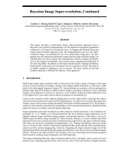
Fig. 3. Representative samples <strong>of</strong> positive target images. Note the wide variety <strong>of</strong><br />
positive images that are all examples <strong>of</strong> a black dot on a white background.<br />
3.1 Tra<strong>in</strong><strong>in</strong>g Data<br />
A subset <strong>of</strong> the positive tra<strong>in</strong><strong>in</strong>g images is shown <strong>in</strong> Figure 3. These were acquired<br />
from a series <strong>of</strong> tra<strong>in</strong><strong>in</strong>g videos us<strong>in</strong>g a simple track<strong>in</strong>g algorithm that was<br />
manually reset on failure. These samples <strong>in</strong>dicate the large variations that occur<br />
<strong>in</strong> real-world scenes. The w<strong>in</strong>dow size was set at 12×12 pixels, which limited<br />
the sample dot size to between 4 and 9 pixels <strong>in</strong> diameter; larger dots are scaled<br />
down by a factor <strong>of</strong> two until they fall with<strong>in</strong> the specification. Samples were<br />
rotated and lightened or darkened to artificially <strong>in</strong>crease the variation <strong>in</strong> the<br />
tra<strong>in</strong><strong>in</strong>g set. This proves to be a more effective means <strong>of</strong> <strong>in</strong>corporat<strong>in</strong>g rotation<br />
and light<strong>in</strong>g <strong>in</strong>variance than ad hoc <strong>in</strong>tensity normalization, as discussed <strong>in</strong> §5.<br />
3.2 Cascad<strong>in</strong>g Classifier<br />
The target location problem here is firmly cast as one <strong>of</strong> statistical pattern classification.<br />
The criteria for choos<strong>in</strong>g a classifier are speed and reliability: the four<br />
subsampled scales <strong>of</strong> a 720×576 pixel video frame conta<strong>in</strong> 522,216 subw<strong>in</strong>dows<br />
requir<strong>in</strong>g classification. Similar to [2], we have adopted a system <strong>of</strong> two cascad<strong>in</strong>g<br />
probes:<br />
– fast Bayes decision rule classification on sets <strong>of</strong> two pixels from every w<strong>in</strong>dow<br />
<strong>in</strong> the frame<br />
– slower, more specific nearest neighbour classifier on the subset passed by the<br />
first stage<br />
The first stage <strong>of</strong> the cascade must run very efficiently, have a near-zero false<br />
negative rate (so that any true positives are not rejected prematurely) and pass<br />
a m<strong>in</strong>imal number <strong>of</strong> false positives. The second stage provides very high classification<br />
accuracy, but may <strong>in</strong>cur a higher computational cost.<br />
3.3 Cascade Stage One: Ideal Bayes<br />
The first stage <strong>of</strong> the cascade constructs an ideal Bayes decision rule from the<br />
positive and negative tra<strong>in</strong><strong>in</strong>g data distributions. These were measured from<br />
the tra<strong>in</strong><strong>in</strong>g data and additional positive and negative images taken from the<br />
tra<strong>in</strong><strong>in</strong>g videos. The sampl<strong>in</strong>g procedure selects two pixels from each subw<strong>in</strong>dow:<br />
one at the centre <strong>of</strong> the dot and the other on the background. The distribution<br />
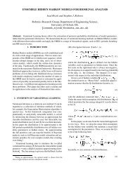
<strong>of</strong> the tra<strong>in</strong><strong>in</strong>g data is shown <strong>in</strong> Figure 4.
1<br />
Edge pixel <strong>in</strong>tensity<br />
Center pixel <strong>in</strong>tensity<br />
Edge pixel <strong>in</strong>tensity<br />
Center pixel <strong>in</strong>tensity<br />
Sensitivity<br />
0.8<br />
0.6<br />
0.4<br />
0.2<br />
0<br />
0 0.2 0.4 0.6 0.8 1<br />
1 − Specificity<br />
(a) (b) (c) (d)<br />
Edge pixel <strong>in</strong>tensity<br />
Center pixel <strong>in</strong>tensity<br />
Fig. 4. Distribution <strong>of</strong> (a) negative pairs g n and (b) positive pairs g p used to construct<br />
the fast classifier. (c) ROC curve used to determ<strong>in</strong>e the value <strong>of</strong> α (<strong>in</strong>dicated by the<br />
dashed l<strong>in</strong>e) which will produce the optimal decision surface given the costs <strong>of</strong> positive<br />
and negative errors. (d) The selected Bayes decision surface.<br />
The two distributions can be comb<strong>in</strong>ed to yield a Bayes decision surface. If g p<br />
and g n represent the positive and negative distributions then the classification<br />
<strong>of</strong> a given <strong>in</strong>tensity pair x is:<br />
{ +1 if α · gp (x) > g<br />
classification(x) =<br />
n (x)<br />
(1)<br />
−1 otherwise<br />
where α is the relative cost <strong>of</strong> a false negative over a false positive. The parameter<br />
α was varied to produce the ROC curve shown <strong>in</strong> Figure 4c. A weight<strong>in</strong>g <strong>of</strong><br />
α = e 12 produces the decision boundary shown <strong>in</strong> Figure 4d, and corresponds<br />
to a sensitivity <strong>of</strong> 0.9965 and a specificity <strong>of</strong> 0.75.<br />
A subw<strong>in</strong>dow is marked as a possible fiducial if a series <strong>of</strong> <strong>in</strong>tensity pairs all<br />
lie with<strong>in</strong> the positive decision region. Each pair conta<strong>in</strong>s the central po<strong>in</strong>t and<br />
one <strong>of</strong> seven outer pixels. The outer edge pixels were selected to m<strong>in</strong>imize the<br />
number <strong>of</strong> false positives based on the above emiprical distributions.<br />
The first stage <strong>of</strong> the cascade seeks dark po<strong>in</strong>ts surrounded by lighter backgrounds,<br />
and thus functions is like a well-tra<strong>in</strong>ed edge detector. Note however<br />
that the decision criteria is not simply (edge − center) > threshold as would be<br />
the case if the center was merely required to be darker than the outer edge. Instead,<br />
the decision surface <strong>in</strong> Figure 4d encodes the fact that {dark center,dark<br />
edge} are more likely to be background, and {light center, light edge} are rare <strong>in</strong><br />
the positive examples. Even at this early edge detection stage there are benefits<br />
from <strong>in</strong>clud<strong>in</strong>g learn<strong>in</strong>g <strong>in</strong> the algorithm.<br />
3.4 Cascade Stage Two: Nearest Neighbour<br />
Among the various methods <strong>of</strong> supervised statistical pattern recognition, the<br />
nearest neighbour rule [18] achieves consistently high performance [19]. The<br />
strategy is very simple: given a tra<strong>in</strong><strong>in</strong>g set <strong>of</strong> examples from each class, a new<br />
sample is assigned the class <strong>of</strong> the nearest tra<strong>in</strong><strong>in</strong>g example. In contrast with<br />
many other classifiers, this makes no a priori assumptions about the distributions<br />
from which the tra<strong>in</strong><strong>in</strong>g examples are drawn, other than the notion that<br />
nearby po<strong>in</strong>ts will tend to be <strong>of</strong> the same class.
For a b<strong>in</strong>ary classification problem given sets <strong>of</strong> positive and negative examples<br />
{p i } and {n j }, subsets <strong>of</strong> R d where d is the dimensionality <strong>of</strong> the <strong>in</strong>put<br />
vectors (144 for the image w<strong>in</strong>dows tested here). The NN classifier is then formally<br />
written as<br />
classification(x) = −sign(m<strong>in</strong> ‖p i − x‖ 2 − m<strong>in</strong> ‖n j − x‖ 2 ) . (2)<br />
i<br />
j<br />
This is extended <strong>in</strong> the k-NN classifier, which reduces the effects <strong>of</strong> noisy tra<strong>in</strong><strong>in</strong>g<br />
data by tak<strong>in</strong>g the k nearest po<strong>in</strong>ts and assign<strong>in</strong>g the class <strong>of</strong> the majority. The<br />
choice <strong>of</strong> k should be performed through cross-validation, though it is common<br />
to select k small and odd to break ties (typically 1, 3 or 5).<br />
One <strong>of</strong> the chief drawbacks <strong>of</strong> the nearest neighbour classifier is that it is<br />
slow to execute. Test<strong>in</strong>g an unknown sample requires comput<strong>in</strong>g the distance<br />
to each po<strong>in</strong>t <strong>in</strong> the tra<strong>in</strong><strong>in</strong>g data; as the tra<strong>in</strong><strong>in</strong>g set gets large this can be a<br />
very time consum<strong>in</strong>g operation. A second disadvantage derives from one <strong>of</strong> the<br />
technique’s advantages: that a priori knowledge cannot be <strong>in</strong>cluded where it is<br />
available. We address both <strong>of</strong> these <strong>in</strong> this paper.<br />
Speed<strong>in</strong>g Up Nearest Neighbour There are many techniques available for<br />
improv<strong>in</strong>g the performance and speed <strong>of</strong> a nearest neighbour classification [20].<br />
One approach is to pre-sort the tra<strong>in</strong><strong>in</strong>g sets <strong>in</strong> some way (such as kd-trees [21]<br />
or Voronoi cells [22]), however these become less effective as the dimensionality<br />
<strong>of</strong> the data <strong>in</strong>creases. Another solution is to choose a subset <strong>of</strong> the tra<strong>in</strong><strong>in</strong>g<br />
data such that classification by the 1-NN rule (us<strong>in</strong>g the subset) approximates<br />
the Bayes error rate [19]. This can result <strong>in</strong> significant speed improvements<br />
as k can now be limited to 1 and redundant data po<strong>in</strong>ts have been removed<br />
from the tra<strong>in</strong><strong>in</strong>g set. These data modification techniques can also improve the<br />
performance through remov<strong>in</strong>g po<strong>in</strong>ts that cause mis-classifications.<br />
We exam<strong>in</strong>ed two <strong>of</strong> the many techniques for obta<strong>in</strong><strong>in</strong>g a tra<strong>in</strong><strong>in</strong>g subset:<br />
condensed nearest neighbour [23] and edited nearest neighbour [24]. The condensed<br />
nearest neighbour algorithm is a simple prun<strong>in</strong>g technique that beg<strong>in</strong>s<br />
with one example <strong>in</strong> the subset and recursively adds any examples that the subset<br />
misclassifies. Drawbacks to this technique <strong>in</strong>clude sensitivity to noise and no<br />
guarantee <strong>of</strong> the m<strong>in</strong>imum consistent tra<strong>in</strong><strong>in</strong>g set because the <strong>in</strong>itial few patterns<br />
have a disproportionate affect on the outcome. Edited nearest neighbour<br />
is a reduction technique that removes an example if all <strong>of</strong> its neighbours are <strong>of</strong> a<br />
s<strong>in</strong>gle class. This acts as a filter to remove isolated or noisy po<strong>in</strong>ts and smooth<br />
the decision boundaries. Isolated po<strong>in</strong>ts are generally considered to be noisy;<br />
however if no a priori knowledge <strong>of</strong> the data is assumed then the concept <strong>of</strong><br />
noise is ill-def<strong>in</strong>ed and these po<strong>in</strong>ts are equally likely to be valid. In our tests it<br />
was found that attempts to remove noisy po<strong>in</strong>ts decreased the performance.<br />
The condens<strong>in</strong>g algorithm was used to reduce the size <strong>of</strong> the tra<strong>in</strong><strong>in</strong>g data<br />
sets as it was desirable to reta<strong>in</strong> “noisy” po<strong>in</strong>ts. Manual selection <strong>of</strong> an <strong>in</strong>itial<br />
sample was found to <strong>in</strong>crease the generalization performance. The comb<strong>in</strong>ed<br />
(test and tra<strong>in</strong><strong>in</strong>g) data was condensed from 8506 positive and 19,052 negative<br />
examples to 37 positive and 345 negative examples.
Parameterization <strong>of</strong> Nearest Neighbour Another enhancement to the nearest<br />
neighbour classifier <strong>in</strong>volves favour<strong>in</strong>g specific tra<strong>in</strong><strong>in</strong>g data po<strong>in</strong>ts through<br />
weight<strong>in</strong>g [25]. In cases where the cost <strong>of</strong> a false positive is greater than the cost<br />
<strong>of</strong> a false negative it is desirable to weight all negative tra<strong>in</strong><strong>in</strong>g data so that<br />
negative classification is favoured. This cost parameter allows a ROC curve to<br />
be constructed, which is used to tune the detector based on the relative costs <strong>of</strong><br />
false positive and negative classifications.<br />
We def<strong>in</strong>e the likelihood ratio to be the ratio <strong>of</strong> distances to the nearest<br />
negative and positive tra<strong>in</strong><strong>in</strong>g examples:<br />
likelihood ratio = nearest negative/nearest positive .<br />
In the vic<strong>in</strong>ity <strong>of</strong> a target dot there will be a number <strong>of</strong> responses where this<br />
ratio is high. Rather than return<strong>in</strong>g all pixel locations above a certa<strong>in</strong> threshold<br />
we locally suppress all non-maxima and return the po<strong>in</strong>t <strong>of</strong> maximum likelihood<br />
(similar to the technique used <strong>in</strong> Harris corner detection [26]; see [27] for<br />
additional details).<br />
4 Implementation<br />
Implementation <strong>of</strong> the cascad<strong>in</strong>g classifier described <strong>in</strong> the previous section is<br />
straightforward; this section describes the target verification step. Figure 2c<br />
shows a typical example <strong>of</strong> the classifier output, where the true positive responses<br />
are accompanied by a small number <strong>of</strong> false positives. Verification is<br />
merely used to identify the target amongst the positive classification responses;<br />
we outl<strong>in</strong>e one approach but there are any number <strong>of</strong> suitable techniques.<br />
First we compute the Delaunay triangulation <strong>of</strong> all po<strong>in</strong>ts to identify the l<strong>in</strong>es<br />
connect<strong>in</strong>g each positive classification with its neighbours. A weighted average<br />
adaptive threshold<strong>in</strong>g <strong>of</strong> the pixels along each l<strong>in</strong>e identifies those with dark<br />
ends and light midsections. All other l<strong>in</strong>es are removed; po<strong>in</strong>ts that reta<strong>in</strong> two<br />
or more connect<strong>in</strong>g l<strong>in</strong>es are passed to a geometric check. This check takes sets <strong>of</strong><br />
four po<strong>in</strong>ts, computes the transformation to map three <strong>of</strong> them onto the corners<br />
<strong>of</strong> a unit right triangle, and then applies that transformation to the rema<strong>in</strong><strong>in</strong>g<br />
po<strong>in</strong>t. If the mapped po<strong>in</strong>t is close enough to the fourth corner <strong>of</strong> a unit square<br />
then retrieve the orig<strong>in</strong>al grayscale image for each fiducial and return the set <strong>of</strong><br />
weighted centroid target coord<strong>in</strong>ates.<br />
5 Discussion<br />
The <strong>in</strong>tention <strong>of</strong> this work was to produce a fiducial detector which <strong>of</strong>fered<br />
extremely high reliability <strong>in</strong> real-world problems. To evaluate this algorithm, a<br />
number <strong>of</strong> video sequences were captured with a DV camcorder and manually<br />
marked up to provide ground truth data. The sequences were chosen to <strong>in</strong>clude<br />
the high variability <strong>of</strong> <strong>in</strong>put data under which the algorithm is expected to be
Sensitivity<br />
(true positives/total positives)<br />
1<br />
0.8<br />
0.6<br />
0.4<br />
0.2<br />
Learnt detector<br />
Normalized<br />
Eng<strong>in</strong>eered<br />
0<br />
0 0.01 0.02 0.03 0.04 0.05<br />
False positives per frame<br />
(a)<br />
Sensitivity<br />
(true positives/total positives)<br />
0.96<br />
0.95<br />
0.94<br />
Learnt detector<br />
Normalized<br />
0 0.01 0.02 0.03 0.04 0.05<br />
False positives per frame<br />
Fig. 5. (a) ROC curve for the overall fiducial detector. The vertical axis displays the<br />
percentage <strong>of</strong> ground truth targets that were detected. (b) An enlarged view <strong>of</strong> the<br />
portion <strong>of</strong> (a) correspond<strong>in</strong>g to the typical operat<strong>in</strong>g range <strong>of</strong> the learnt detector. The<br />
drop <strong>in</strong> detection rate at 0.955 is an artefact <strong>of</strong> the target verification stage whereby<br />
some valid targets are rejected due to encroach<strong>in</strong>g false positive fiducials.<br />
(b)<br />
used. It is important also to compare performance to a traditional “eng<strong>in</strong>eered”<br />
detector, and one such was implemented as described <strong>in</strong> the appendix.<br />
The fiducial detection system was tested on six video sequences conta<strong>in</strong><strong>in</strong>g<br />
<strong>in</strong>door/outdoor light<strong>in</strong>g, motion blur and oblique camera angles. The reader is<br />
encouraged to view the video <strong>of</strong> detection results available from [28].<br />
Ground truth target coord<strong>in</strong>ates were manually recorded for each frame and<br />
compared with the results <strong>of</strong> three different detection systems: learnt classifier,<br />
learnt classifier with subw<strong>in</strong>dow normalization, and the eng<strong>in</strong>eered detector<br />
described <strong>in</strong> the appendix. Table 1 lists the detection and false positive rates<br />
for each sequence, while Table 2 lists the average number <strong>of</strong> positives found<br />
per frame. Overall, the fast classification stage returned just 0.33% <strong>of</strong> the subw<strong>in</strong>dows<br />
as positive, allow<strong>in</strong>g the classification system to process the average<br />
720×576 frame at four scales <strong>in</strong> 120 ms. The operat<strong>in</strong>g range is up to 10 m with<br />
a 50 mm lens and angles up to 75 degrees from the target normal.<br />
Normaliz<strong>in</strong>g each subw<strong>in</strong>dow and classify<strong>in</strong>g with normalized data was shown<br />
to <strong>in</strong>crease the number <strong>of</strong> positives found. The target verification stage must then<br />
exam<strong>in</strong>e a larger number <strong>of</strong> features; s<strong>in</strong>ce this portion <strong>of</strong> the system is currently<br />
implemented <strong>in</strong> Matlab alone it causes the entire algorithm to run slower. This is<br />
added to the <strong>in</strong>creased complexity <strong>of</strong> comput<strong>in</strong>g the normalization <strong>of</strong> each subw<strong>in</strong>dow<br />
prior to classification. By contrast, append<strong>in</strong>g a normalized copy <strong>of</strong> the<br />
tra<strong>in</strong><strong>in</strong>g data to the tra<strong>in</strong><strong>in</strong>g set was found to <strong>in</strong>crease the range <strong>of</strong> classification<br />
without significantly affect<strong>in</strong>g the number <strong>of</strong> false positives or process<strong>in</strong>g time.<br />
The success rate on the dimly lit bar sequence was <strong>in</strong>creased from below 50% to<br />
89.3% by <strong>in</strong>clud<strong>in</strong>g tra<strong>in</strong><strong>in</strong>g samples normalized to approximate dim light<strong>in</strong>g.
Table 1. Success rate <strong>of</strong> target verification with various detectors. Normaliz<strong>in</strong>g each<br />
w<strong>in</strong>dow prior to classification improves the success rate on some frames, but more false<br />
positive frames are <strong>in</strong>troduced and the overall performance is worse. The eng<strong>in</strong>eered<br />
detector cannot achieve the same level <strong>of</strong> reliability as the learnt detector.<br />
Learnt Normalized Eng<strong>in</strong>eered<br />
detector detector detector<br />
Sequence Targets True False True False True False<br />
Church 300 98.3% 2.0% 99.3% 8.7% 46.3% 0.0%<br />
Lamp 200 95.5% 0.5% 99.5% 3.0% 61.5% 0.0%<br />
Lounge 400 98.8% 0.5% 96.5% 1.0% 96.5% 0.0%<br />
Bar 975 89.3% 0.0% 91.3% 0.0% 65.7% 0.5%<br />
Multiple 2100 95.2% 0.7% 93.5% 3.5% 83.0% 1.4%<br />
Library 325 99.1% 0.6% 94.2% 0.0% 89.8% 5.2%<br />
Summary 4300 94.7% 0.4% 94.0% 2.3% 77.3% 1.1%<br />
Careful quantitative experiments compar<strong>in</strong>g this system with the AR Toolkit<br />
(an example <strong>of</strong> a developed method <strong>of</strong> fiducial detection) have not yet been<br />
completed, however a qualitative analysis <strong>of</strong> several sequences conta<strong>in</strong><strong>in</strong>g both<br />
targets under a variety <strong>of</strong> scene conditions has been performed. Although the<br />
AR Toolkit performs well <strong>in</strong> the <strong>of</strong>fice, it fails under motion blur and when <strong>in</strong>camera<br />
light<strong>in</strong>g disrupts the b<strong>in</strong>arization. The template match<strong>in</strong>g to identify a<br />
specific target does not <strong>in</strong>corporate any colour or <strong>in</strong>tensity normalization and is<br />
therefore very sensitive to light<strong>in</strong>g changes. We deal with all <strong>of</strong> these variations<br />
through the <strong>in</strong>clusion <strong>of</strong> relevant tra<strong>in</strong><strong>in</strong>g samples.<br />
This paper has presented a fiducial detector which has superior performance<br />
to reported detectors. This is because <strong>of</strong> the use <strong>of</strong> mach<strong>in</strong>e learn<strong>in</strong>g. This detector<br />
demonstrated 95% overall performance through <strong>in</strong>door and outdoor scenes<br />
Table 2. Average number <strong>of</strong> positive fiducial classifications per frame. The full classifier<br />
is only applied to the positive results <strong>of</strong> the fast classifier. This cascade allows the learnt<br />
detector to run faster and return fewer false positives than the eng<strong>in</strong>eered detector.<br />
True Fast Full Normalized Eng<strong>in</strong>eered<br />
Sequence positives classifier classifier full classifier detector<br />
Church 4 5790 107 135 121<br />
Lamp 4 560 23 30 220<br />
Lounge 4 709 36 55 43<br />
Bar 4 82 5 6 205<br />
Multiple 7.3 † 2327 79 107 96<br />
Library 4 1297 34 49 82<br />
Average - 1794 47 64 128<br />
† The Multiple sequence conta<strong>in</strong>s between 1 and 3 targets per frame.
<strong>in</strong>clud<strong>in</strong>g multiple scales, background clutter and motion blur. A cascade <strong>of</strong><br />
classifiers permits high accuracy at low computational cost.<br />
The primary conclusion <strong>of</strong> the paper is the observation that even “simple”<br />
vision tasks become challeng<strong>in</strong>g when high reliability under a wide range <strong>of</strong><br />
operat<strong>in</strong>g conditions is required. Although a well eng<strong>in</strong>eered ad hoc detector<br />
can be tuned to handle a wide range <strong>of</strong> conditions, each new application and<br />
environment requires that the system be more or less re-eng<strong>in</strong>eered. In contrast,<br />
with appropriate strategies for manag<strong>in</strong>g tra<strong>in</strong><strong>in</strong>g set size, a detector based on<br />
learn<strong>in</strong>g can be retra<strong>in</strong>ed for new environments without significant architectural<br />
changes.<br />
Further work will exam<strong>in</strong>e additional methods for reduc<strong>in</strong>g the computational<br />
load <strong>of</strong> the second classifier stage. This could <strong>in</strong>clude Locally Sensitive<br />
Hash<strong>in</strong>g as a fast approximation to the nearest neighbour search, or a different<br />
classifier altogether such as a support vector mach<strong>in</strong>e.<br />
References<br />
1. Kle<strong>in</strong>, G., Drummond, T.: Tightly <strong>in</strong>tegrated sensor fusion for robust visual track<strong>in</strong>g.<br />
In: Proc. BMVC. Volume 2. (2002) 787 –796<br />
2. Viola, P., Jones, M.: Rapid object detection us<strong>in</strong>g a boosted cascade <strong>of</strong> simple<br />
features. In: Proc. CVPR. (2001)<br />
3. Neumann, U., Bajura, M.: Dynamic registration correction <strong>in</strong> augmented-reality<br />
systems. In: IEEE Virtual Reality Annual Int’l Symposium. (1995) 189–196<br />
4. Welch, G., et al.: The HiBall tracker: High-performance wide-area track<strong>in</strong>g for<br />
virtual and augmented environments. In: Proc. ACM VRST. (1999) 1–10<br />
5. Mellor, J.P.: Enhanced reality visualization <strong>in</strong> a surgical environment. A.I. Technical<br />
Report 1544, MIT, Artificial Intelligence Laboratory (1995)<br />
6. State, A., et al.: Superior augmented reality registration by <strong>in</strong>tegrat<strong>in</strong>g landmark<br />
track<strong>in</strong>g and magnetic track<strong>in</strong>g. In: SIGGRAPH. (1996) 429–438<br />
7. Cho, Y., Neumann, U.: Multi-r<strong>in</strong>g color fiducial systems for scalable fiducial track<strong>in</strong>g<br />
augmented reality. In: Proc. <strong>of</strong> IEEE VRAIS. (1998)<br />
8. Scharste<strong>in</strong>, D., Briggs, A.: Real-time recognition <strong>of</strong> self-similar landmarks. Image<br />
and Vision Comput<strong>in</strong>g 19 (2001) 763–772<br />
9. Rekimoto, J., Ayatsuka, Y.: Cybercode: Design<strong>in</strong>g augmented reality environments<br />
with visual tags. In: Proceed<strong>in</strong>gs <strong>of</strong> DARE. (2000)<br />
10. Kato, H., Bill<strong>in</strong>ghurst, M.: Marker track<strong>in</strong>g and hmd calibration for a video-based<br />
augmented reality conferenc<strong>in</strong>g system. In: Int’l Workshop on AR. (1999) 85–94<br />
11. Owen, C., Xiao, F., Middl<strong>in</strong>, P.: What is the best fiducial? In: The First IEEE<br />
International Augmented Reality Toolkit Workshop. (2002) 98–105<br />
12. de Ip<strong>in</strong>a, D.L., et al.: Trip: a low-cost vision-based location system for ubiquitous<br />
comput<strong>in</strong>g. Personal and Ubiquitous Comput<strong>in</strong>g 6 (2002) 206–219<br />
13. Naimark, L., Foxl<strong>in</strong>, E.: Circular data matrix fiducial system and robust image<br />
process<strong>in</strong>g for a wearable vision-<strong>in</strong>ertial self-tracker. In: ISMAR. (2002)<br />
14. Efrat, A., Gotsman, C.: Subpixel image registration us<strong>in</strong>g circular fiducials. International<br />
Journal <strong>of</strong> Computational Geometry and Applications 4 (1994) 403–422<br />
15. Bruckste<strong>in</strong>, A.M., Holt, R.J., Huang, T.S., Netravali, A.N.: New devices for 3D<br />
pose estimation: Mantis eyes, Agam pa<strong>in</strong>t<strong>in</strong>gs, sundials, and other space fiducials.<br />
International Journal <strong>of</strong> Computer Vision 39 (2000) 131–139
16. Wellner, P.: Adaptive threshold<strong>in</strong>g for the digital desk. Technical Report EPC-<br />
1993-110, Xerox (1993)<br />
17. Malbez<strong>in</strong>, P., Piekarski, W., Thomas, B.: Measur<strong>in</strong>g ARToolkit accuracy <strong>in</strong> long<br />
distance track<strong>in</strong>g experiments. In: 1st Int’l AR Toolkit Workshop. (2002)<br />
18. Cover, T., Hart, P.: Nearest neighbor pattern classification. IEEE Trans. Information<br />
Theory 13 (1967) 57–67<br />
19. Ripley, B.D.: Why do nearest-neighbour algorithms do so well? SIMCAT (Similarity<br />
and Categorization), Ed<strong>in</strong>burgh (1997)<br />
20. Wilson, D.R., Mart<strong>in</strong>ez, T.R.: Reduction techniques for <strong>in</strong>stance-based learn<strong>in</strong>g<br />
algorithms. Mach<strong>in</strong>e Learn<strong>in</strong>g 38 (2000) 257–286<br />
21. Sproull, R.F.: Ref<strong>in</strong>ements to nearest-neighbor search<strong>in</strong>g <strong>in</strong> k-dimensional trees.<br />
Algorithmica 6 (1991) 579–589<br />
22. Berchtold, S., Ertl, B., Keim, D.A., Kriegel, H.P., Seidl, T.: Fast nearest neighbor<br />
search <strong>in</strong> high-dimensional spaces. In: Proc. ICDE. (1998) 209–218<br />
23. Hart, P.: The condensed nearest neighbor rule. IEEE Trans. Information Theory<br />
14 (1968) 515–516<br />
24. Duda, R., Hart, P., Stork, D.: Pattern Classification. 2nd edn. John-Wiley (2001)<br />
25. Cost, S., Salzberg, S.: A weighted nearest neighbor algorithm for learn<strong>in</strong>g with<br />
symbolic features. Mach<strong>in</strong>e Learn<strong>in</strong>g 10 (1993) 57–78<br />
26. Harris, C., Stephens, M.: A comb<strong>in</strong>ed corner and edge detector. In: Proceed<strong>in</strong>gs<br />
<strong>of</strong> the 4th ALVEY Vision Conference. (1988) 147–151<br />
27. Claus, D.: Video-based survey<strong>in</strong>g for large outdoor environments. First Year<br />
Report, <strong>University</strong> <strong>of</strong> <strong>Oxford</strong> (2004)<br />
28. http://www.robots.ox.ac.uk/˜dclaus/eccv/fiddetect.mpg.<br />
Appendix: Eng<strong>in</strong>eered Detector<br />
One important comparison for this work is how well it compares with traditional<br />
ad hoc approaches to fiducial detection. In this section we outl<strong>in</strong>e a local<br />
implementation <strong>of</strong> such a system.<br />
Each frame is converted to grayscale, b<strong>in</strong>arized us<strong>in</strong>g adaptive threshold<strong>in</strong>g as<br />
described <strong>in</strong> [16], and connected components used to identify cont<strong>in</strong>uous regions.<br />
The regions are split <strong>in</strong>to scale b<strong>in</strong>s based on area, and under or over-sized regions<br />
removed. Regions are then rejected if the ratio <strong>of</strong> the covex hull area and actual<br />
area is too low (region not entirely filled or boundary is not cont<strong>in</strong>ually convex),<br />
or if they are too eccentric (if the axes ratio <strong>of</strong> an ellipse with the same second<br />
moments is too high).