MTH 654 Numerical Methods for Inverse Problems

MTH 654
Numerical Methods for Inverse Problems
Lab 1
Due: Nov 3
The objective of this project is to help students familiarize themselves with the concepts of
paramer estimation problems. In addition, students will practice using MATLAB to carry
out many computations associated with solving inverse problems. Read the model
description, then work either 1 or 2 (Bonus: do both!)
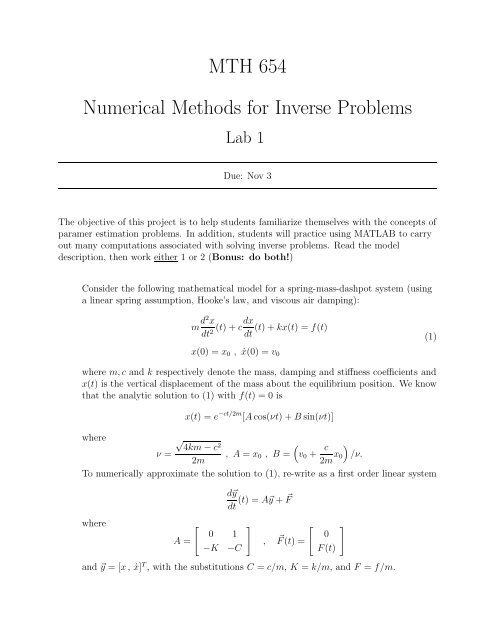
Consider the following mathematical model for a spring-mass-dashpot system (using
a linear spring assumption, Hooke’s law, and viscous air damping):
m d2 x
(t) + cdx(t) + kx(t) = f(t)
dt2 dt (1)
x(0) = x 0 , ẋ(0) = v 0
where m, c and k respectively denote the mass, damping and stiffness coefficients and
x(t) is the vertical displacement of the mass about the equilibrium position. We know
that the analytic solution to (1) with f(t) = 0 is
x(t) = e −ct/2m [A cos(νt) + B sin(νt)]
where
√
4km − c
2
(
ν = , A = x 0 , B = v 0 + c )
2m
2m x 0 /ν.
To numerically approximate the solution to (1), re-write as a first order linear system
where
A =
[
0 1
−K −C
d⃗y
dt (t) = A⃗y + ⃗ F
]
, ⃗ F(t) =
[
0
F(t)
]
and ⃗y = [x, ẋ] T , with the substitutions C = c/m, K = k/m, and F = f/m.

1. Mass-spring-dashpot
(a) Using reasonable values for m, c, k solve the homogeneous system in MATLAB
using the routine of your choice (e.g., ode23, ode45, ode15s, or roll your
own). Plot the numerical solution x h (t) on the same graph as the analytical
solution for some meaningful time interval. Comment on any discrepancies.
On your graph, you should label the horizontal axis as time, t, the vertical axis
as x(t), and place in the title of the graph a text string showing values of m, c,
and k (sprintf may be helpful).
(b) In this exercise, we will create “simulated” data to be used for estimating the
unknown parameters. Use the analytic solution to generate discrete data
x j = x(t j ) on a meaningful interval [0, T] at M equally-spaced time points
Use, for example M = 100.
t j =
jT
M − 1 .
(c) Define a least squares objective function for the inverse problem to determine
parameters ⃗q = [C, K] given data ⃗x and appropriate initial conditions (known).
Use a numerical solution method to compare to data (although an analytic
solution is possible for this model, it is not available in general).
(d) Using several “nearby” initial guesses, and several “other” initial guesses, apply
a black box optimization routine to minimize the least squares functional. I
recommend lsqnonlin, but note that it wants the residuals, not the sum of the
squares of residuals. Feel free to use any package you are familiar with. Report
in a table the initial guess, initial cost, final estimate, final cost, and either the
computation time required to get the estimate or the number of function
evaluations required. Comment on any failures.
(e) In practice, the data collected is corrupted by noise (for example, errors in
collecting data, instrumental errors, etc.). In the next part of the exercise, we
wish to test the sensitivity of the inverse least squares method to errors in
sampling the data. For this, we will add to each simulated datum an error term
as follows. Artificially add noise to your data with noise level (i.e., standard
deviation) b by
d j = x j + η j
where η j ∼ N(0, b 2 ). In MATLAB this is d=x+b*rand(M,1);.
(f) Choose one initial estimate from 1d, and a variety of increasing noise levels
(starting at zero, e.g. 0, 0.01, 0.05, 0.1), and solve the inverse problem again,
reporting results in a table as before. Additionally, make a plot of the minimum
objective function value as a function of noise level. Describe the sensitivity of
the inverse least squares method with respect to the noise level b.
(g) Finally, compute the confidence interval for each of the estimates from 1f. Plot
estimates for C with confidence intervals as a function of noise level (see
errorbar). Repeat for K. Comment on what you observe.

2. Vibrating Beam
Download BeamData.mat from the course website and run load BeamData in
MATLAB. This will create variables Td and Ad which contain accelerometer data
collected from a vibrating beam which was excited at its first fundamental frequency
(approximately 11 Hz). The data is truncated to a time point at which acceleration is
zero (use this to determine the initial position!). See Figure 1 for an idealized picture.
2
Accelerometer data
1.5
1
0.5
x’’ (m/s 2 )
0
−0.5
Begin Collect Data
−1
−1.5
Stop Forcing
−2
0 5 10 15 20 25 30
t (s)
Figure 1: Beam Excitation: Shown is idealized accelerometer data from a vibrating beam.
Sinusoidal input is stopped at t = 10, data collection begins at t = 15 where ẍ = 0.
We will use the mass-spring-dashpot model in (1) to attempt to represent the
dynamics of the beam data.
(a) Plot Ad versus Td to visualize the data.
(b) Formulate the least squares parameter identification problem for ⃗q = [C, K, v 0 ]
using acceleration data.
(c) Solve this inverse problem using the black box optimization routine of your
choice, for example, lsqnonlin or fminsearch (Bonus: use both and
compare results!). Use a numerical solution method to compare to data (see
1a). Do not take the derivative of your solution to the ODE to get the
acceleration, but rather, plug x and ẋ into the ODE. For an initial guess, try

any three numbers of your choice (note C ≥ 0 and K ≥ 0). Report your initial
guess, initial cost, final estimate and final cost. Plot the acceleration
corresponding to your final estimate on the same plot as the data. Just for fun,
try other random initial guesses. Does there seem to be a local minimum to the
objective function that has a very large basin of attraction? (Feel free to make a
surface plot, or better yet, a volumetric plot (see slice) if you’re interested.)
(d) Solve the inverse problem again with an initial guess in the vicinity of
[0.002, 1.3, 4850]. Report your initial guess, initial cost, final estimate and final
cost. Plot the acceleration corresponding to your final estimate on the same plot
as the data. Describe any discrepancy in your final solution versus the data.
Explain why there may be this discrepancy.
(e) Repeat 2d with the assumption that C = 0 in the model.
(f) Use the χ 2 (1) test to test for the significance of your improved fit to the data by
allowing nontrivial damping C ≠ 0 in the model. State in terms of a Null and
Alternate Hypothesis. Does your answer make sense from looking at the data?
Explain why or why not.