A Model of Open-Baffle Loudspeakers - DIY Audio Projects

A Model of Open-Baffle Loudspeakers
5025 (H-6)
Juha Backman
Nokia Mobile Phones
FIN-00045 Nokia Group, Finland
Presented at
the 107th Convention
1999 September 24-27
New York
This preprint has been reproduced from the author’s advance
manuscript, without editing, corrections or consideration by the
Review Board. The AES takes no responsibility for the
contents.
Additional preprints may be obtained by sending request and
remittance to the Audio Engineering Society, 60 East 42nd St.,
New York, New York 10165-2520, USA.
All rights reserved. Reproduction of this preprint, or any portion
thereof, is not permitted without direct permission from the
Journal of the Audio Engineering Society.
AN AUDIO ENGINEERING
SOCIETY PREPRINT

0 Abstract
A Model of Open-Baffle Loudspeakers
Juha Backman
Nokia Mobile Phones
P.O. Box 100
Nokia Group
Finland
E-mail: juha.backman@nokia.com
The open-baffle loudspeaker is, although structurally very simple, a challenge for modelling. This
paper presents a computationally efficient model for predicting the frequency response and the
polar pattern of an open-baffle loudspeaker. The baffle is modelled using time-domain geometrical
theory of diffraction, and the conventional driver model is complemented with simple additions to
approximate the acoustical asymmetry of the structure.
1 Introduction
Open-baffle loudspeakers are the longest-known1 and structurally simplest loudspeakers, but they,
at the same time, pose considerable theoretical challenges for the modelling. A simple dipole model
partially explains some of their features, but such a model is valid only at very low frequencies, and
the parameters of the model (e.g. the effective size of the dipole) are difficult to determine. The
simple dipole model fails in several respects: it is impossible to take into account asymmetry and
other baffle shape effects, the mid-frequency polar pattern is not predicted correctly, etc. Thus
taking into account both driver properties and baffle geometry is needed.
The open-baffle speakers do, in addition to being theoretically interesting, have some practical
importance. Dipole loudspeakers (and other gradient loudspeakers) provide a constant directivity
also at low frequencies. They also excite fewer low-frequency room modes (although the benefit of
this is not self-evident) and their acoustical power output is affected by side boundaries much less
than the output of omnidirectional speakers*.
Despite these advantages the open-baffle speakers are far from being ideal woofers. Their wellknown
practical problem is their inability to produce adequate low-frequency output. This is a
problem particularly with electrostatic and ribbon units (which otherwise are not being discussed
within this paper), where the displacement is limited, and there is a trade-off between the
displacement and the sensitivity. Larger volume velocities can be achieved by using dynamic
woofers, but to maximise their output, a baffle is needed around the driver. The low frequency
(dimensions (( a) output of a dipole is proportional to both the volume velocity and the linear
dimensions, so doubling the baffle size equals doubling the displacement. This baffle in turn creates
’ HUNT, FREDERIK V.: Electroacoustics. The Analysis of Transduction, and Its Historical Background. Harvard
University Press, 1954; reprint Acoustical Society of America, 1982, pp. 86 - 87.
* MORSE, PHILIP M.; INGAARD, K. UNO: Theoretical Acoustics, McGraw-Hill, Inc., New York, 1968; reprint Princeton
University Press, Princeton, 1986, pp. 372 - 375.
1

easily problems with mid-frequency response and polar pattern, thus losing the advantages of the
open baffle and constraining the usable frequency range.
2 Computational model
2.1 Overview
The open-baffle loudspeaker discussed in this paper consists of a rigid, flat baffle and a circular
driver (or multiple drivers) placed at an arbitrary location on the baffle. If only first-order scattering
is being studied, the only formal constraint on the baffle shape is that the edge is at least almost
convex (i.e. a straight line drawn outwards from the source encounters the edge only at one point;
some global concavity is allowed, so far as this condition is fulfilled). When multiple scattering is
computed, then the baffle edge has to be convex. Of course in practice only few simple geometries
are encountered. The acoustical behaviour of the baffle is described by using time-domain
geometrical theory of diffraction, considering both sides separately; important observation that
simplifies the analysis is that if the driver is assumed to be symmetrical, then the signal impinging
on the edge is identical, but of opposite phase. If simple geometries are considered, then analytical
expressions or simple closed-form approximations can be obtained for the impulse responses.
The driver can be regarded to operate almost independently of the acoustical load provided by the
baffle, and thus a frequency-domain lumped-component description is appropriate. A significant
aspect of the driver function, regarding especially open-baffle applications, is the acoustical
asymmetry provided by the chassis, etc. A simple approximation for the asymmetry, which
improves the accuracy of predicting mid-frequency polar pattern and response, is to model the
chassis as a Hehnholtz resonator, which then acts as an acoustical low-pass filter for the rear side of
the driver.
For the purposes of creating an efficient model for the open-baffle speaker, several simplifying
assumptions need to be made:
- baffle is thin enough as compared to the wavelength in order to be regarded as infinitely
thin. In practice this limits the validity of the model to baffles thinner than about W4.
- the radiation from the driver can be approximated by a rigid, circular piston. The frequency
responses of the front and rear sides, however, need not be identical (section 2.9, although
a symmetrical driver enables further simplification of the model.
- baffle vibration is ignored. This does not affect the accuracy of the diffraction model, but
as the baffle area may be much larger than the driver area, the baffle vibration can have a
great practical significance.
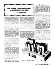
According to these assumptions, the radiation consists of three components (Figure 1):
- direct sound from the driver
- sound radiated from the front of the driver and scattered from the edges
- sound radiated from the rear of the driver and scattered from the edges
The direct sound can be calculated effectively; the challenges are in determining the near-field
sound caused by the driver at the edge and the field scattered from this sound.

Edge
scattering
from f?ont
Direct sound
Edge
scattering
from re&
Driver
J
L
Baffle
Figure 1. The components of sound radiated by a speaker in a finite open baffle. As indicated
below, the scattering strength is determined by the angle 8 measured from the front surface of the
baffle.
We start by analysing the diffraction
between the edge point
of sound emitted by a point source in a baffle. The distance
Figure 2. Parameters for describing a point source on a rectangular baffle.
Angle CJ.I can be as a function of time in the form
Equation 1
cp = arccosi
The diffracted sound can be represented by directional secondary sources distributed along the edge
of the baffle. The strength of the source can be determined by applying the principle of reciprocity
and the angular dependence of the sound scattered from an edge point to an angle 8 in a plane
normal to the edge can be expressed by an equation presented by Vanderkooy3, which for a thin
knife-edge wedge simplifies to
Equation 2 W) = cosnJy~~s(j,2 = -co;(.j,2
3 VANDERKOOY, JOHN: A Simple Theory of Cabinet Edge Diffraction. JAES, vol. 39, December 1991, pp. 923 - 933;
reprinted in the AES Anthology Loudspeakers, vol. 3, pp. 230 - 242.
3

The shortcoming of this form is that its behaviour near the shadow edge is problematic, but both the
illuminated and the shadow regions themselves, especially near the loudspeaker axis, behave rather
well.
The sound pressure created at distance r by the radiation Corn an edge surrounding an open baffle
loudspeaker consists of the contributions of the positive and the negative side,
Equation 3 p = pd;;;dtF(e) + pd;;;dtF(2w9)= pd;;;dt-co$,2 +pd~;;dtcos;,2
If the driver can be regarded as symmetrical, as usually at low frequencies, then the scattered sound
pressure can be simplified to the form
Equation 4 p = - pdqfdt 2
4nr case/2
When the observation point is not in the normal plane of the edge, then the sound pressure is to be
multiplied by a factor 1 /co& where c is the angle between the propagation direction and the normal
plane.
2.2 Near-field radiation
Although the general near-field radiation problem is notoriously difficultd, especially when the
calculations are performed in the frequency domain, the problem can be simplified greatly for the
purposes of the computation of diffraction. When the field point is constrained to the same plane as
the surface of the piston, approximate frequency-domain calculation of the radiation can be done
relatively efficiently. In the time domain the situation is even more interesting, since the radiation
can be represented by a simple exact expression.
I ,-- Driver
Field point
(baffle edge)
Figure 3. Geometry used in determining the near-field radiation.
The sound pressure dp generated by an area element dA on a piston vibrating with velocity u is
4 STENZEL, H.: tier die Berechung des Schallfeldes von kreisfirmigen Membranen in starrer Wand, Annalen der
Physik, vol. 6, n:o 4, 1949, pp. 303 - 324.
4

Equation 5
dp =--=PdudA, P dq
4x?? dt
4nR dt
where R is the distance between the field point and the element dA. The distance can be also written
as R = ct, where t is the propagation time and c the speed of sound.
The surface points corresponding to the sound received at time t form an arc with a radius ct (Figure
3). The area of the surface element is dA = ctd@dt, which implies that the total sound radiated at
time t is
Equation 6 p =
‘I2 pdufdt
I
-912 4nzt
ctd@ =
pdu I dt
4x
e-
The angle @ can be shown to be
Equation 7
$ = arccos
d2 + (ct)2 - a2
2ctd ’
from which the sound pressure can be written as
Equation 8
duldt
p = -
4x
d2 + (ct)2 - a2
arccos ,(d-a)lc

1
0.9
0.8
3 0.7
Ti 5 0.6
u 0.5
8
z 0.4
8 E 0.3
0.2
0.1
0
-0.6 -0.4 -0.2 0 0.2 0.4 0.6
Time
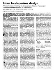
Figure 4. Impulse response at different distance from the source (normalised to the maximum
value): solid line: distance = 2 times driver radius, dashed line: distance = 3 times driver radius,
dotted line: distance = 5 times driver radius, dash-dot line: distance = 100 times driver radius.
If the model is used calculate the behaviour of a free piston (a totally unbaffled speaker), then the
radiation model will be numerically difficult (a division by zero) just at the edge. (Analytically, the
limiting value can be still shown to be correct.) The numerical difficulties can be circumvented e.g.
by assuming a very narrow annular baffle around the driver.
2.3 Multiple scattering
For qualitative description of mid-frequency behaviour, the multiple scattering effects can be
ignored. Vanderkooy has demonstrated in his papers, however, that taking multiple scattering is
essential for describing low frequencies accurately. As shown later, the effect is even more
pronounced for open-baffle speakers. To simplify the analysis the edge is represented again by a
discrete set of points. The geometry of baffle has now to be limited to convex shapes, however,
since a sound propagating between any arbitrary edge points has to stay inside (or on) the edge.
When calculating multiple scattering the sound propagating on both sides of the baffle has to be
taken into account.
5 VANDEERKOY, ref. 3.

Figure 5. Schematic representation of multiple scattering. Thick solid line = first sound from driver
to edge; solid thin line = second-order scattering; dashed line = third-order scattering.
Although the multiple scattering process can be from signal processing point of view regarded to be
an IIR filter, representing it as a conventional filter will result in a rather complex and thus memoryconsuming
network. An alternative way is to represent the signal an edge point as a polynomial of z-
’ and to use a matrix representation for the multiple scattering:
Equation 10
Pl
P2
a1,2 ’ a3,2 a 42
P3 = al,3 a2,3 0 an,3
.
. .
. . .
P n-N+1 Ul,tl a2,n a34 *** 0
Pl
P2
P3
PVl
where N is the order of scattering; N = 1 is the first sound arriving from the driver to the edge point.
Each matrix element a,, consists of a real coefficient representing the scattering amplitude from
point i toj and an exponential z-~(‘~)“, where D(ij) is the distance between the points. In practice the
distance (divided by c) can be truncated to the closest integer value to keep the computation simple.
If the baffle has straight edges, then the scattering coefficient between any points on the same edge
is zero. The multiple scattering matrix is independent of the driver size or position.
The multiplication of the vector consisting of the polynomials by the matrix resembles the
convolution of the two; the delays represented matrix, however, are not uniformly spaced or
consecutively ordered in each column. Each multiplication corresponds to an operation of delaying
and attenuating the sample. The operation could be turned into a proper convolution by arranging
each column of the matrix by the power of z-‘, merging elements corresponding to the same power
and writing the result as an impulse response.
Each scattering naturally lengthens the impulse response. The number of samples added can be
estimated simply from the maximum dimension of the baffle. For a 1 * 1 m2 baffle the length of the
diagonal is about 1.4 m, which at 100 kHz sampling rate equals about 412 samples. Thus, after 5
scatterings the original impulse response is lengthened only about by 2000 samples.

2.4 Far-field radiation
2.4.1 Radiation from the driver
As far as the direct sound only is concerned, the driver can be regarded to reside in an infinite, flat
plane. This approximation can be used even with completely free pistons, since the diffracted part is
taken separately into account. There are two ways of representing the far-field direct radiation from
a rigid piston: in frequency domain and in time domain. The frequency-domain expression for the
sound pressure created by a piston vibrating with a volume velocity q and a frequencyfat distance r
and angle 8 can be represented by the familiar expression6
zypq 2 J1 (ka sin 0)
Equation 11 p = --
r kasine
and the time-domain radiation corresponding to a step displacement A by the following
equationy:
Equation 12 p =
r-ct
a2 sin2 8 - (r - ct)2
ct

problematic in the actual implementation of the algorithm, since the non-causal part of the energy is
small, and since there will be some initial delay from the propagation from the source to the edge
point, even windowing away the part causing non-causality in the final result will not have a strong
effect on the energy.
After the delays and amplitudes corresponding to each edge point have been determined, then the
impulse responses on each edge point are delayed and attenuated by the appropriate amount and
added. If fractional delays are used, then this involves explicitly convolving the delay and the
impulse response. The use of fractional delays will increase the computation per edge point, but the
number of points will be reduced, which reduces the computational load at earlier stages and
reduces the amount of memory needed.
The polar pattern can be obtained by computing the frequency response to several angles and
tracking the behaviour of a single frequency. An alternative way, which is faster if only a few
frequencies are computed, is to go back to the definition of the Fourier transform and compute the
inner product of the impulse response to the desired angles with sinusoidals corresponding to the
desired frequencies. This yields the spectrum component at that particular frequency. As the
magnitude of the transfer function is needed, then for each frequency the multiplication should be
done with both a sine and a cosine signal, yielding the imaginary and the real parts.
2.5 Practical drivers
When the frequency range of interest goes well above the fundamental resonance of the driver, the
structural asymmetry of a typical transducer must be taken into account. In typical loudspeakers a
simple approximation for the structure is to model the volume between the diaphragm and the
chassis and the chassis holes as a Hehnholtz resonator. The practical problem of this kind of model
is that the effective port length becomes difficult to determine computationally, since the distance
between the holes and the diaphragm is roughly similar to the dimensions of the holes, and the
baffle hole etc. will influence the effective length. The Hehnholtz resonator model, however, gives
a reasonable qualitative approximation for the asymmetry in the frequency response, although the
asymmetry of the radiation pattern (both near-field and far-field) is still ignored.
Port formed by chassis
holes and baffle
Volume
between
diaphragm and
chassis
Figure 6. Geometrical parameters describing the Helmholtz resonator approximation for the rear of
the driver.

Bli
Figure 7. Simple equivalent circuit of a driver, using a Helmholtz resonator to describe the
structural asymmetry.
One interesting feature of the simple model described here is that it qualitatively explains why an
unbaffled or open-baffle loudspeaker becomes almost omnidirectional at some frequency band in
the midrange. Near and above the Helmholtz resonance frequency the driver and chassis port
velocities are almost in phase (Figure 8), so the cancellation between front and rear radiation is
reduced (and at right angle the sound from both sides is in phase), which typically creates a wider
radiation pattern than the driver would have had at the same frequency in an infinite baffle or a
sealed enclosure. The optimum condition for omnidirectional radiation (about equal magnitudes,
small phase difference) occurs slightly above the Helmholtz resonance frequency.
10

a)
/ Frequency/Hz
0
%
a, b -50
P
8
5
g-100
.-
-0
%
E-150
b)
-200
10’ lo2 -IO3 lo4
Frequency/Hz
Figure 8. Magnitude (a) of the sound pressure radiated by the front (solid) and rear (dashed) sides a
speaker described by the equivalent circuit in Figure 7 and the phase difference between the front
and the rear radiation (b). In this example the fundamental resonance is at 100 Hz and the chassis
Hehnholtz resonance at 2 kHz.
Using this kind of model the acoustical asymmetry can be regarded as a factor independent of the
diffraction and the radiation. Thus impulse responses using an idealised source (with a flat response
in the far-field on-axis in an infinite baffle) can be used to model the diffraction and the direct
sound in the time domain, and the responses can then be transformed into frequency domain to be
multiplied by the driver responses and finally to be added (Figure 9).
11

Front diffraction Total front FFT Driver front
for ideal piston --) radiation (TD) + + frequency
VW response (FD)
h
Rear diffraction
for ideal piston
0-D)
Total rear
radiation (TD)
Added to front or rear
i observation direction
FFT
Driver rear
frequency
response (FD)
Total radiation
0-j
A
Figure 9. Steps in calculating the total response taking into account the driver properties. TD = time
domain calculation, FD = frequency domain calculation.
In practical design work a it is possible to mount the driver in a large baffle (significantly larger
than the target size of the final design) or a wall, with a large space behind it, and to measure the
near-field impulse response in the plane of the baffle at some distance(s) appropriate for the
intended final design. The measurements have to be performed for the both sides of the driver using
a baffle as thick as the one to be used in the final design, since the baffle thickness affects strongly
the asymmetry of the radiation.
The radiation load (for the purposes of this model, mainly attached mass) changes slightly when the
driver is in a finite baffle, and thus the resonance is frequency between the free-air and the infinitebaffle
values. This can be taken into account by starting with the idealised piston model and
calculating the average diffracted sound pressure across the driver on the other side; this yields then
a term comparable to the mutual radiation impedance between the driver sides. The correction is
small, however.
3 Low-frequency approximation
At very low frequencies the open baffle starts to behave as an ideal dipole, exhibiting the figure-ofeight
polar pattern and the additional 6 dB/oct. attenuation as compared to the same driver in an
infinite baffle. This low-frequency limit determines the choice of driver parameters (resonance
frequency, Q) needed. The radiation of an ideal dipole can be determined from two parameters:
volume velocity of the individual monopoles comprising the dipole and their distance. The effective
distance is determined from the baffle size and the placement of the driver. As the numerical
example in the next section indicates, however, the first-order scattering model yields too low an
amplitude at the low frequencies and too high a frequency for the first minimum, which would
suggest that the effective distance should be determined from a series expansion describing the
multiple scattering.
The effective distance can be assumed to be average distance from the centre of the driver to the
edge, calculating the average over the angle measured from the driver (Figure 10). This type of
averaging is justified by noting that the sound energy is radiated from the driver to all directions in
about the same manner, so the angle averaging equals energy averaging.
12

Figure 10. The parameters describing the average distance from the edge.
For a rectangular baffle the distance can be written as
Equation 13 r(0) = & ,
where r, is the distance from the edge under study and 8 the angle calculated for that particular
edge. If the edge is delimited by angles 8,,, and 0,,, then the average distance is
Equation 14
Taking the uppermost edge as an example, the minimum and maximum angles for an edge can be
defined from the geometry of the baffle as
Equation 15
X0
%in = -arcsin
x0” +Y;
0 = arcsin Xl ’
max
x: +Y:
from which the average distance for this particular edge can be written as
Equation 16 rave, r =
1
11
Xl X0
arcsin + arcsin
xf +yo2 4 +Yo2
Repeating this for other edges yields the total average distance, from which can be computed the
estimate for the on-axis sound pressure at distance r
. 2
Equation 17 p = zp~~~
13

where 4 is the volume velocity corresponding to one side of the driver.
The frequency of the first minimum (on-axis) is according to this model
Equation 18 fti
= c
r ave
4 Numerical example
The results obtained by the method are illustrated by the results obtained from the baffle illustrated
below (Figure 11).
300
< >
Figure 11. The
200
T
0100
-: ” L
100
-l
400
baffle used in the examples (all dimensions in mm).
0.4 ,
0.35 -
43
.z 0.3 -
-6
kii 0.25 -
8
6 0.2-
5:
!!? 0.15-
1
2 0.1 -
z
0.05 -
o-
0 0.001 0.002 0.003 0.004 0.0050.006 0.007 0.008 0.009 0.01
Time/s
Figure 12. Impulse response of the first-order scattered sound.
14

0.025,
I
$ 0.02 -
3
.z
E 0.015-
crs
8
g 0.01 -
z:
f!J
a, 0.005 -
u,
2
E o- \ ”
-0.005 I
0 0.001 0002 0 003 0.004 0.005 0.006 0.007 0.008 0.009 0.01
Time/s
Figure
order,
13. Impulse response of the scattered sound, taking into account the scattering up to Sh
An interesting feature is that the average decay characteristics are almost perfectly exponential
(Figure 14).
-20
-40
-60 t
%
3i -80 -
2 -100 -
"a
fii -120 -
E-,40
3
-
2 -160 -
6
-180 -
0 0.001 0.002 0.003 0.004 0.005 0.006 0.007 0.008 0.009 0.01
Time/s
Figure 14. Decay characteristics of the scattered sound, plotted on a logarithmic scale.
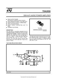
The importance of multiple scattering is clearly illustrated from the frequency responses calculated
using the impulse responses shown above. (The edge impulse response is subtracted from the direct
sound, if the sign of the diffracted sound is chosen as illustrated; in a physical system the sign of the
diffracted sound in the illuminated region is opposite to the direct sound, and in the shadow region
the same.) The response predicted using only single diffraction indicates too much low-frequency
attenuation and too large local minima and maxima in the response.
15

5
0
%
B
3
g
E
a -5
/
.
. . .
. \
. . .
. . .
. . . .
-10
lo2
IO3
Frequency/Hz
lo4
Figure 15. Frequency response corresponding to 1 St-order scattering (dashed line) and Sh-order
scattering (solid line).
5 Conclusions
The method presented here enables a fast calculation of the characteristics of an unbaffled
loudspeaker. The model is quite usable for calculating the frequency response up to angles
approaching the shadow boundary, but is problematic in predicting the behaviour at the plane of the
baffle. The numerical simulations shown indicate clearly that multiple scattering has to be taken
into account.
16