A Family of Wavelets and ...
A Family of Wavelets and ...
A Family of Wavelets and ...

Create successful ePaper yourself
Turn your PDF publications into a flip-book with our unique Google optimized e-Paper software.
Revista da Sociedade Brasileira de Telecomunicações<br />
Volume xx Número XX, xxxxx 2xxxx<br />
( deO )<br />
( deO )<br />
Denoting by s ( t ) ↔ S ( w ) the corresponding<br />
transform pair, it follows that ( deO ) ( deO ) 1<br />
ψ ( t ) = s ( t − ) .<br />
2<br />
The shaping pulse can be rewritten as:<br />
( )<br />
⎛ 1 π (1 + α)<br />
⎞<br />
2π<br />
S deO ( w)<br />
= PCOS⎜w;<br />
, − , π , πα ⎟ +<br />
⎝ 4α<br />
4α<br />
⎠<br />
⎛ 3π<br />
α π ⎞ ⎛ 1 2π<br />
(1 − α)<br />
⎞<br />
PCOS⎜<br />
w;0,0,<br />
(1 − ), (1 − 3α<br />
) ⎟ + PCOS⎜w;<br />
, − ,2π<br />
,2πα<br />
⎟<br />
⎝ 2 3 2 ⎠ ⎝ 8α<br />
8α<br />
⎠<br />
Figure 8. Modulo <strong>of</strong> "de Oliveira" Wavelet on frequency<br />
domain varying the roll-<strong>of</strong>f parameter (depth axis).<br />
Finally, applying the inverse transform, we have<br />
( ) ⎛ 1 π (1 + α)<br />
⎞<br />
2π<br />
s deO ( t)<br />
= pcos⎜t;<br />
, − , π , πα ⎟ +<br />
(17)<br />
⎝ 4α<br />
4α<br />
⎠<br />
⎛ 3π<br />
α π ⎞ ⎛ 1 2π<br />
(1 − α)<br />
⎞<br />
pcos⎜t;0,0,<br />
(1 − ), (1 − 3α<br />
) ⎟ + pcos⎜t;<br />
, − ,2π<br />
,2πα<br />
⎟<br />
⎝ 2 3 2 ⎠ ⎝ 8α<br />
8α<br />
⎠<br />
The pcos(.) signal is a complex signal when there are no<br />
symmetries in PCOS(.). The real <strong>and</strong> imaginary parts <strong>of</strong> the<br />
pcos function can be h<strong>and</strong>led separately, according to<br />
pcos ( t;t0 , θ 0 ,w0<br />
,B) = rpcos( t) + j.ipcos( t)<br />
, where<br />
rpcos( t) : = R e( pcos( t;t0 , θ 0 ,w0<br />
,B))<br />
<strong>and</strong><br />
ipcos( t) : = Im( pcos( t;t0 , θ 0 ,w0<br />
,B))<br />
.<br />
Aiming to investigate the wavelet behaviour, we propose to<br />
separate the Real <strong>and</strong> Imaginary parts <strong>of</strong> s (deO) (t),<br />
introducing new functions rpc(.) <strong>and</strong> ipc(.)<br />
( deO ) ⎧ ( deO ) 1 ⎫ ( deO ) ⎧ ( deO ) 1 ⎫<br />
R e ( t ) = Re<br />
s ( t − ) I mψ ( t ) = Im<br />
s (t − )<br />
. (18)<br />
ψ<br />
, { }<br />
⎨<br />
⎩<br />
⎬<br />
2 ⎭<br />
∆ w ( + ) : = w0<br />
+ B<br />
⎨<br />
⎩<br />
⎬<br />
2 ⎭<br />
∆w ( −1 ) : = w0<br />
− ;<br />
Proposition 2. Let<br />
1 <strong>and</strong> B<br />
1<br />
∆ θ ( + )<br />
: = Bt0<br />
+ w0t0<br />
+θ <strong>and</strong> ( 1<br />
0 ∆θ − )<br />
: = Bt0<br />
− w0t0<br />
−θ be auxiliary<br />
0<br />
parameters. Then<br />
rpc<br />
ipc<br />
1<br />
2π<br />
− t .<br />
0<br />
∑<br />
sen ∆θ<br />
( i )<br />
( i )<br />
cos ∆w<br />
t + t.<br />
i∈{<br />
−1,<br />
+ 1}<br />
i∈{<br />
−1,<br />
+ 1}<br />
( t) =<br />
,<br />
− t0.<br />
1<br />
sen ∆θ<br />
( i )<br />
2<br />
2<br />
0<br />
t − t<br />
( i )<br />
sen ∆w<br />
t + t.<br />
∑<br />
( i )cos ∆θ<br />
( i )<br />
sen ∆w<br />
i∈{<br />
−1,<br />
+ 1}<br />
i∈{<br />
−1,<br />
+ 1}<br />
( t) =<br />
.<br />
2π<br />
∑<br />
2<br />
2<br />
0<br />
t − t<br />
∑<br />
( −i<br />
)cos ∆θ<br />
( i )<br />
( i )<br />
cos ∆w<br />
Pro<strong>of</strong>. Follows from trigonometry identities.<br />
At this point, an alternative notation<br />
( + 1 ) ( −1<br />
) ( + 1 ) ( −1<br />
)<br />
rpc( t ) = rpc( t; ∆w<br />
, ∆w<br />
, ∆θ , ∆θ<br />
)<br />
<strong>and</strong><br />
( + 1)<br />
( −1)<br />
( + 1 ) ( −1)<br />
ipc( t ) = ipc( t; ∆w<br />
, ∆w<br />
, ∆θ , ∆θ<br />
) can be introduced<br />
to explicit the dependence on these new parameters.<br />
( )<br />
H<strong>and</strong>ling apart the real <strong>and</strong> imaginary parts <strong>of</strong> s deO ( t)<br />
, we<br />
arrive at<br />
( deO )<br />
( s ( t ))<br />
⎛<br />
π ⎞<br />
2π Re<br />
= rpc⎜t;<br />
π(<br />
1 + α ), π(<br />
1 − α ), 0,<br />
⎟ +<br />
⎝<br />
2 (19)<br />
⎠<br />
⎛<br />
π ⎞<br />
rpc( t; 2π<br />
( 1 − α ), π(<br />
1 + α ), 0,<br />
0) + rpc⎜t;<br />
2π<br />
( 1 + α ), 2π<br />
( 1 − α ), , 0⎟.<br />
⎝<br />
2 ⎠<br />
t<br />
( i )<br />
t<br />
❏<br />
Applying now proposition 2, after many algebraic<br />
manipulations:<br />
( deO)<br />
2π<br />
R e s ( t)<br />
( ) =<br />
1 1−α<br />
2(1+<br />
α<br />
{ Η ( ) ( ) ( )<br />
)<br />
2(1−α<br />
)<br />
t − Η<br />
(1+<br />
α )<br />
t + Μ1+<br />
α<br />
t + Μ<br />
2(1−α<br />
)<br />
( t)<br />
}<br />
2<br />
<strong>and</strong><br />
( deO)<br />
( deO)<br />
Re( ψ ( t)<br />
) = Re( s ( t −1/<br />
2) ).<br />
= , (20)<br />
The analysis <strong>of</strong> the imaginary part can be done in a<br />
similar way.<br />
Definition 3. (Special functions); ν is a real number,<br />
cos( νπt<br />
)<br />
Hν ( t ) : = ν , 0≤ν≤1, <strong>and</strong><br />
νπt<br />
ν 1 2 | ν1<br />
−ν<br />
|<br />
( t ) :<br />
[ ] { sin t ( )t.cos t}<br />
1<br />
2<br />
Μν<br />
=<br />
πν<br />
2 1 − 2 ν<br />
2<br />
1 −ν<br />
2 πν ❏<br />
2<br />
π 1−<br />
2t(<br />
ν1<br />
−ν<br />
2 )<br />
The imaginary part <strong>of</strong> the wavelet can be found mutatus<br />
mut<strong>and</strong>i:<br />
( deO )<br />
2π I m( s ( t )) =<br />
1−α<br />
2(<br />
1+<br />
α )<br />
= { Η2(<br />
1−α<br />
)( t ) − Η(<br />
1+<br />
α )( t ) + Μ1+<br />
α ( t ) + Μ2<br />
( 1−α<br />
)( t )}<br />
2<br />
( deO)<br />
( deO)<br />
<strong>and</strong> Im( ψ ( t)<br />
) = Im( s ( t −1/<br />
2) ).<br />
1 , (21)<br />
The real part (as well as the imaginary part) <strong>of</strong> the<br />
(<br />
complex wavelet ψ deO ) ( t ) are plotted in figure 9, for<br />
α =0.1, 0.2 <strong>and</strong> 1/3.<br />
Re<br />
Im<br />
( deO )<br />
( ψ ( t ))<br />
( deO )<br />
( ψ ( t ))<br />
(<br />
Figure 9. Wavelet ψ<br />
deO ) ( t ) : (a) real part <strong>of</strong> the wavelet<br />
<strong>and</strong> (b) imaginary part <strong>of</strong> the wavelet. (Sketches for α = 0.1,<br />
0.2 <strong>and</strong> 1/3). The effective support <strong>of</strong> such wavelets is the<br />
interval [-12,12].<br />
(a)<br />
(b)<br />
5