Biostatistics 209, Lab #3 Discussion
Biostatistics 209, Lab #3 Discussion
Biostatistics 209, Lab #3 Discussion

Create successful ePaper yourself
Turn your PDF publications into a flip-book with our unique Google optimized e-Paper software.
<strong>Biostatistics</strong> <strong>209</strong>, <strong>Lab</strong> <strong>#3</strong> <strong>Discussion</strong><br />
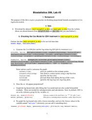
3. Checking the Cox Model for ZDV treatment in lab3-actg019_a.dta<br />
a. Generate the Cox-KM plot and the log-minus-log KM plot by ZDV.<br />
b. Does the rx HR appear proportional?<br />
Here we look to see if the log-minus-log curves display a constant distance apart.<br />
Instead, we see the two curves coming together. This pattern is typical of a large<br />
treatment effect that fades over time. However, it is difficult to discern from this<br />
graph how quickly the treatment effect diminishes.<br />
c. Graph the log hazard ratio after fitting the Cox model and save the scaled Schoenfeld<br />
residuals. These are needed for subsequent plots and calculations. Recall, ZDV is the<br />
reference group for the variable rx.<br />
d. Re-graph the log hazard ratio with a lowess smoother, and save the lowess values in the<br />
variable named “smloghr” (obviously you can call it something else).<br />
1
<strong>Biostatistics</strong> <strong>209</strong> <strong>Lab</strong> #2<br />
Cox regression -- Breslow method for ties<br />
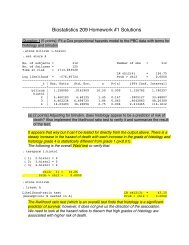
No. of subjects = 880 Number of obs = 880<br />
No. of failures = 55<br />
Time at risk = 354872<br />
LR chi2(1) = 5.66<br />
Log likelihood = -328.57534 Prob > chi2 = 0.0174<br />
------------------------------------------------------------------------------<br />
_t | Haz. Ratio Std. Err. z P>|z| [95% Conf. Interval]<br />
-------------+----------------------------------------------------------------<br />
rx | 1.957118 .5719375 2.30 0.022 1.103739 3.470304<br />
------------------------------------------------------------------------------<br />
Placebo subjects on average have about 2 times hazard of HIV progression compared to<br />
subjects on ZDV.<br />
Note the difference in the smoothers (seen in the two different graphs); the running mean<br />
smoother on the left is rather flat, as running mean smoothers tend to be. The lowess<br />
shows a more pronounced trajectory. In the lowess graph, we can see that the log HR<br />
decreases with time, which indicates violations of proportional hazards. I have included in<br />
the this graph a flat reference line at log(1.96) = 0.67. If hazards were truly proportional the<br />
lowess line should approximate a flat line. It does not.<br />
e. Look at the graph and the variable smloghr and fill in the following table.<br />
log HR<br />
HR<br />
95 days (3 mos) 1.71 5.52<br />
181 days (6 mos) 1.46 4.31<br />
362 days (12 mos) 0.71 2.03<br />
540 days (18 mos) 0.19 1.21<br />
2
<strong>Biostatistics</strong> <strong>209</strong> <strong>Lab</strong> #2<br />
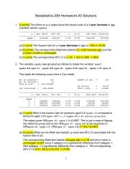
f. Run the Schoenfeld test for the proportional hazards assumption. Is there evidence against<br />
that? Does this agree with the plots?<br />
Test of proportional-hazards assumption<br />
Time: Time<br />
----------------------------------------------------------------<br />
| rho chi2 df Prob>chi2<br />
------------+---------------------------------------------------<br />
rx | -0.30819 5.39 1 0.0202<br />
------------+---------------------------------------------------<br />
The test agrees closely with the plots in concluding that there is a clear violation of<br />
proportional hazards. The HRʼs over time appear quite different despite the p-value=0.02<br />
is not overwhelmingly so. This reflects the moderate sample size (55 events).<br />
g. How would you summarize the effect of ZDV on progression of HIV?<br />
Tests and graphical examination showed that the effect of ZDV violated the<br />
assumption of proportional hazards (p=0.02); that is, the effect of ZDV decreased over<br />
time. Subjects taking placebo had HIV progression risk about 5.5, 4.3 and 2.0 times<br />
higher than subjects taking ZDV at 3, 6 and 12 months, respectively. The effect<br />
appeared to decrease steadily and by 18 months, progression rates were only 20%<br />
higher on placebo compared with ZDV.<br />
However, be aware that choosing a different bandwidth (default bwidth=0.8) would<br />
change the values in the table, e.g.<br />
lowess giveAname days, bwidth(.5) generate(smloghr)<br />
log HR<br />
HR<br />
95 days (3 mos) 1.70 5.48<br />
181 days (6 mos) 1.67 5.32<br />
362 days (12 mos) 0.61 1.83<br />
540 days (18 mos) 0.23 1.25<br />
3
<strong>Biostatistics</strong> <strong>209</strong> <strong>Lab</strong> #2<br />
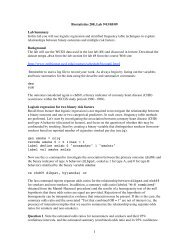
4. Checking the Cox Model for Cholesterol in lab3-pbc_a.dta<br />
a. Fit the Cox model for the effect of cholesterol and run the Schoenfeld test for the<br />
proportional hazards assumption. Does the evidence appear against the assumption?<br />
No. of subjects = 284 Number of obs = 284<br />
No. of failures = 114<br />
Time at risk = 1908.583167<br />
LR chi2(1) = 6.37<br />
Log likelihood = -565.65984 Prob > chi2 = 0.0116<br />
------------------------------------------------------------------------------<br />
_t | Haz. Ratio Std. Err. z P>|z| [95% Conf. Interval]<br />
-------------+----------------------------------------------------------------<br />
cholest | 1.000758 .0002714 2.79 0.005 1.000226 1.00129<br />
------------------------------------------------------------------------------<br />
Test of proportional-hazards assumption<br />
Time: Time<br />
----------------------------------------------------------------<br />
| rho chi2 df Prob>chi2<br />
------------+---------------------------------------------------<br />
cholest | 0.29729 7.77 1 0.0053<br />
------------+---------------------------------------------------<br />
The test indicates a violation of proportional hazards with a p-value of 0.005.<br />
However, we need to look at the graph to understand the nature of the violation.<br />
b. Graph the log hazard ratio. What does the graph suggest? Do you have any concerns<br />
about the test?<br />
The graph shows two large outliers, which appears to be greatly affecting the<br />
correlations with time. These two values may have a large effect on the test of<br />
proportional hazards. You would want to redo the test without these points.<br />
c. Try deleting some potential influential points and then re-run the plot and test for the<br />
proportional hazards assumption. What do you conclude?<br />
First, to fully re-run you either had to use a different stub in the sca( ) option or<br />
drop the variable you named it before.<br />
4
<strong>Biostatistics</strong> <strong>209</strong> <strong>Lab</strong> #2<br />
No. of subjects = 266 Number of obs = 266<br />
No. of failures = 112<br />
Time at risk = 1338.001372<br />
LR chi2(1) = 8.15<br />
Log likelihood = -537.48194 Prob > chi2 = 0.0043<br />
------------------------------------------------------------------------------<br />
_t | Haz. Ratio Std. Err. z P>|z| [95% Conf. Interval]<br />
-------------+----------------------------------------------------------------<br />
cholest | 1.001022 .0003138 3.26 0.001 1.000407 1.001637<br />
------------------------------------------------------------------------------<br />
Test of proportional-hazards assumption<br />
Time: Time<br />
----------------------------------------------------------------<br />
| rho chi2 df Prob>chi2<br />
------------+---------------------------------------------------<br />
cholest | 0.15694 2.31 1 0.1282<br />
------------+---------------------------------------------------<br />
Here, we see that deleting the two points made the violation of proportional hazards<br />
no longer significant (p>0.05). This is further<br />
reinforced by the graph, although it shows some<br />
possible evidence against proportional hazards.<br />
For example, you can try<br />
estat phtest, detail rank<br />
estat phtest, detail log<br />
The bottom line is that the test of proportional hazards can be greatly affected by outlying<br />
values and it is important to always accompany the test by a graph so that you judge the<br />
directions, the magnitude of the violation and whether there appear to points exerting a<br />
large influence on the test.<br />
5