Lab 3: Handout Quantum-ESPRESSO: a first principles code, part 2.
Lab 3: Handout Quantum-ESPRESSO: a first principles code, part 2.
Lab 3: Handout Quantum-ESPRESSO: a first principles code, part 2.

You also want an ePaper? Increase the reach of your titles
YUMPU automatically turns print PDFs into web optimized ePapers that Google loves.
MIT 3.320 Atomistic Modeling of Materials Spring 2005<br />
1<br />
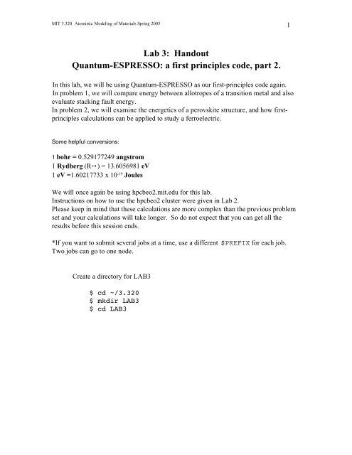
<strong>Lab</strong> 3: <strong>Handout</strong><br />
<strong>Quantum</strong>-<strong>ESPRESSO</strong>: a <strong>first</strong> <strong>principles</strong> <strong>code</strong>, <strong>part</strong> <strong>2.</strong><br />
In this lab, we will be using <strong>Quantum</strong>-<strong>ESPRESSO</strong> as our <strong>first</strong>-<strong>principles</strong> <strong>code</strong> again. <br />
In problem 1, we will compare energy between allotropes of a transition metal and also<br />
evaluate stacking fault energy. <br />
In problem 2, we will examine the energetics of a perovskite structure, and how <strong>first</strong>-<br />
<strong>principles</strong> calculations can be applied to study a ferroelectric.<br />
Some helpful conversions:<br />
1 bohr = 0.529177249 angstrom<br />
1 Rydberg (R ) = 13.6056981 eV<br />
1 eV =1.60217733 x 10 -19 Joules<br />
We will once again be using hpcbeo<strong>2.</strong>mit.edu for this lab. <br />
Instructions on how to use the hpcbeo2 cluster were given in <strong>Lab</strong> <strong>2.</strong><br />
Please keep in mind that these calculations are more complex than the previous problem<br />
set and your calculations will take longer. So do not expect that you can get all the<br />
results before this session ends.<br />
*If you want to submit several jobs at a time, use a different $PREFIX for each job.<br />
Two jobs can go to one node.<br />
Create a directory for LAB3<br />
$ cd ~/3.320 <br />
$ mkdir LAB3<br />
$ cd LAB3
MIT 3.320 Atomistic Modeling of Materials Spring 2005<br />
2<br />
Problem 1<br />
Problem 1 will look at calculations involving Cobalt. We will use the LDA<br />
exchange-correlation functional. Since Co is a ferromagnetic material, we will do<br />
spin-polarized calculations. To set up these calculations, you should have a basic<br />
knowledge of crystal structures. Chapter 1 of Introduction to Solid State Physics<br />
by Kittel is a good introduction.<br />
First, Create a directory for PROBLEM1<br />
$ mkdir PROBLEM1<br />
$ cd PROBLEM1<br />
Next, copy files from /home/lee0su/3.320/LAB3/<br />
$ cp ~lee0su/3.320/LAB3/Co.* .<br />
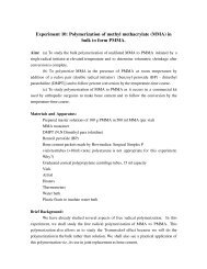
HCP structure<br />
c<br />
b<br />
a<br />
a<br />
Below is a copy of the file Co.HCP.scf.in, along with explanations.<br />
For the sake of brevity, I will not repeat entries which have the same meaning as<br />
the previous handout, except for items which you will be required to change.
MIT 3.320 Atomistic Modeling of Materials Spring 2005<br />
3<br />
(1) &control<br />
(2) calculation = 'scf'<br />
(3) restart_mode='from_scratch'<br />
(4) prefix='Co.HCP'<br />
(5) tstress = .true.<br />
(6) tprnfor = .true.<br />
(7) outdir = '/state/<strong>part</strong>ition1/lee0su'<br />
(8) pseudo_dir = '/state/<strong>part</strong>ition1/lee0su'<br />
(9) /<br />
(10) &system<br />
(11) ibrav= 4<br />
(12) celldm(1) = 1<br />
(13) celldm(3) = 2<br />
(14) nat= 2<br />
(15) ntyp= 1<br />
(16) ecutwfc = 30<br />
(17) ecutrho = 250<br />
(18) starting_magnetization(1) = 0.7<br />
(19) occupations = 'smearing'<br />
(20) degauss = 0.03<br />
(21) smearing = 'cold'<br />
(22) nspin = 2<br />
(23) /<br />
(24) &electrons<br />
(25) mixing_beta = 0.7<br />
(26) conv_thr = 1.0d8<br />
(27) /<br />
(28) ATOMIC_SPECIES<br />
(29) Co 58.933 Co.pzndrrkjus.UPF<br />
(30) ATOMIC_POSITIONS (crystal)<br />
(31) Co 0.3333333333 0.6666666667 0.25<br />
(32) Co 0.6666666667 0.3333333333 0.75<br />
(33) K_POINTS {automatic}<br />
(34) 2 2 1 0 0 0
MIT 3.320 Atomistic Modeling of Materials Spring 2005<br />
4<br />
Line 11<br />
This line contains information about the Bravais lattice. ibrav = 4<br />
refers to the hexagonal lattice. Refer to INPUT_PW to see how each<br />
bravais lattice is defined.<br />
Line 12-14<br />
There are two independent lattice parameters in a hexagonal lattice (as you<br />
probably know). Refer to the figure if you have forgotten how to construct<br />
an HCP structure. celldm(1) is a in bohr ( not angstrom ! ) and<br />
celldm(3) is c/a ( not the absolute value of c ! ). Find an appropriate<br />
value of celldm(3) from your knowledge of the ideal HCP structure.<br />
Two atoms comprise one unit cell.<br />
Line 16-17<br />
We are going to use ultrasoft pseudopotentials here. In the case of normconserving<br />
pseudopotentials, ecutrho (the charge density cutoff) is<br />
automatically determined by 4*ecutwfc. However, in the case of<br />
ultrasoft pseudopotentials, we need an augmented charge around the ion<br />
core, so ecutrho should be higher than 4*ecutwfc.<br />
The usual value is 25-35 Ry for ecutwfc and 200-300 Ry for ecutrho.<br />
You might want to do a convergence check. Keep in mind that the value<br />
you should look at is the energy difference or force, not the absolute value<br />
of the energy (the energy will not converge unless you use very, very high<br />
ecutwfc and ecutrho).<br />
Lines 18<br />
starting_magnetization is the starting magnetization for the<br />
atom. Set this to a value between -1 and +1.<br />
Lines 19-21<br />
These keywords are <strong>part</strong>icular details for the Brillioun zone integration<br />
for metals. Since there is a discontinuity of the occupation number for the<br />
bands around the Fermi energy, total energy with respect to the number<br />
of k-points converges very slowly. Adding electronic temperature<br />
(degauss) smooth out the abrupt change of the occupation number and<br />
as a result total energy converges with fewer number of k-points.<br />
Lines 22<br />
nspin=2 turns ON spin polarization while nspin=1 turns it OFF. We<br />
will use nspin=2 throughout Problem 1.<br />
Lines 30-32<br />
You should be cautious when you set up atomic positions.
MIT 3.320 Atomistic Modeling of Materials Spring 2005<br />
5<br />
Problem 1-1<br />
The default is alat , which means that you are using Cartesian coordinates<br />
and everything is scaled by celldm(1).<br />
In the case of HCP , it is easier to express coordinates with respect to<br />
crystal axes, which are a, b, and c in the figure. This way you don't need to<br />
change the atomic coordinates accordingly whenever you change celldm<br />
(3).<br />
Lines 33<br />
This is k-point information. One thing to keep in mind is since the unit<br />
cell is longer in the c direction, a sparser k-mesh can be used in that<br />
direction.<br />
You should find the correct k-point grid yourself. <br />
There are two scripts, one for FCC and the other for HCP. It should be<br />
straightforward to check k-point convergence using these scripts.<br />
Co.FCC.scf.j<br />
Co.HCP.scf.j ( fixed c/a ratio )<br />
To get total energy vs. k-point mesh, ( e.g. a = 4.74 )<br />
$ grep ! Co.FCC.4.74.30.250.*.out | cut c 2425,6390 > ksum.30.250<br />
To get total energy vs. lattice parameter,<br />
$ grep ! Co.FCC.*.30.250.1<strong>2.</strong>out | cut c 1215,6390 > esum.30.250.12<br />
If you want to do something more complex, refer to<br />
/home/lee0su/3.320/LAB3/getE.sh<br />
Make any necessary changes for your own purpose.<br />
Problem 1-2<br />
To change a and c independently, use<br />
Co.HCP.covera.scf.j<br />
The script is almost the same as Co.HCP.scf.j and self-explanatory.
MIT 3.320 Atomistic Modeling of Materials Spring 2005<br />
6<br />
Problem 1-4<br />
Problem 1-5<br />
To generate FCC structure in hexagonal cell,<br />
Make a small change ( celldm(3), nat ... ) to Co.HCP.scf.j<br />
Set up and run a calculation using Co.HCP.scf.j for a 5-atom cell<br />
ABCAC<br />
Check your result with the automatic script<br />
Co.ABCAC.j<br />
The script will do everything for you, after you specify the lattice parameters and<br />
the number of layers ( $nlayer ). It is very important for you to make an input<br />
file at least once on your own. Spend several minutes trying to understand what is<br />
going on in the script.<br />
Extra credit problem<br />
To get total energy, magnetic moment, and pressure, use<br />
/home/lee0su/3.320/LAB3/getM.sh
MIT 3.320 Atomistic Modeling of Materials Spring 2005<br />
7<br />
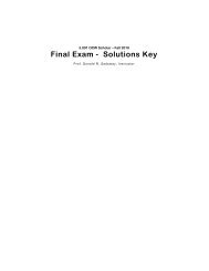
Problem 2<br />
In this problem, we will be looking at BaTiO 3 in the cubic phase and tetragonal<br />
phase. The atomic positions of the cubic perovskite structure are shown below.<br />
Figure 1. Representation of a cubic perovskite structure. In our case, O is<br />
present on each of the faces, Ba on each corner and Ti in the body-centered<br />
position.<br />
Take a look at the file BaTiO3.ion_dynamics_example.in
MIT 3.320 Atomistic Modeling of Materials Spring 2005<br />
8<br />
(1) &control<br />
(2) calculation = 'relax',<br />
(3) restart_mode = 'from_scratch',<br />
(4) prefix = 'BaTiO3',<br />
(5) tstress = .true.,<br />
(6) tprnfor = .true.,<br />
(7) pseudo_dir = '/state/<strong>part</strong>ition1/yourusername/',<br />
(8) outdir = '/state/<strong>part</strong>ition1/yourusername/'<br />
(9) /<br />
(10) &system<br />
(11) ibrav = 1, celldm(1) = 7.5, nat = 5, ntyp = 3,<br />
(12) ecutwfc = 30.0, ecutrho = 240.0<br />
(13) /<br />
(14) &electrons<br />
(15) diagonalization = 'cg',<br />
(16) mixing_mode = 'plain',<br />
(17) mixing_beta = 0.7,<br />
(18) conv_thr = 1.0d8<br />
(19) /<br />
(20) &ions<br />
(21) ion_dynamics = 'bfgs'<br />
(22) /<br />
(23)<br />
(24)ATOMIC_SPECIES<br />
(25) Ba 137.327 Ba.UPF<br />
(26) Ti 47.88 Ti.UPF<br />
(27) O 15.9994 O.UPF<br />
(28)<br />
(29)ATOMIC_POSITIONS<br />
(30) Ba O.0 0.0 0.0 0 0 0<br />
(31) Ti 0.5 0.5 0.5 0 0 0<br />
(32) O 0.5 0.5 0.0<br />
(33) O 0.5 0.0 0.5 <br />
(34) O 0.0 0.5 0.5<br />
(35)<br />
(36)K_POINTS automatic<br />
(37) 4 4 4 1 1 1
MIT 3.320 Atomistic Modeling of Materials Spring 2005<br />
9<br />
Line 2<br />
For <strong>part</strong>s (b) and (c), instead of a single self-consistent field calculation,<br />
we will be doing a 'relax' calculation which includes a series of SCF calculations.<br />
Here, the ions are allowed to move in order to reduce the total system energy.<br />
This setting is very much like setting the 'opti' flag in GULP. Note that for <strong>part</strong><br />
(a), you should use 'scf', as in problem1.<br />
Lines 7-8<br />
Remember to set your scratch directory correctly.<br />
Lines 20-22<br />
Since we will be using ion “dynamics”, we now need the new IONS<br />
section. We are not, however, using real dynamics(i.e. there is no time coordinate<br />
used in the relaxations), but just searching for the minimum energy relaxations.<br />
This section should be omitted for the scf calculations of <strong>part</strong> (a).<br />
Lines 33-34<br />
You will notice that there are now three additional flags at the end of our<br />
atomic coordinates. These flags define the degrees of freedom available for those<br />
atoms during relaxation (zero = disallow motion in that direction for that atom).<br />
In the example shown above, the Ba and Ti ions are fixed, while the O ions are<br />
allowed to relax. So the format is:<br />
atomic label pos_x pos_y pos_z allow_x allow_y allow_z<br />
You will find that using scripts will save you tons of time on this problem set.<br />
Not using scripts would mean that you could spend literally days sitting at a<br />
computer waiting for runs to finish. You should be able to set up the appropriate<br />
scripts based on the ones we've already used for examining Fe and also the<br />
example script from last problem set. If you are still uncomfortable with writing<br />
your own scripts, make an appointment with your TA to work out some basic<br />
scripts for completing this problem set.<br />
A sample shell script for submitting a job using this example input file can be<br />
found in the ~brandonw/LAB3 directory. You should copy this file and modify it<br />
appropriately.