An advanced detrending method with application to HRV analysis ...
An advanced detrending method with application to HRV analysis ...
An advanced detrending method with application to HRV analysis ...

Create successful ePaper yourself
Turn your PDF publications into a flip-book with our unique Google optimized e-Paper software.
1<br />
<strong>An</strong> <strong>advanced</strong> <strong>detrending</strong> <strong>method</strong> <strong>with</strong> <strong>application</strong><br />
<strong>to</strong> <strong>HRV</strong> <strong>analysis</strong><br />
Mika P. Tarvainen, Perttu O. Ranta-aho, and<br />
Pasi A. Karjalainen<br />
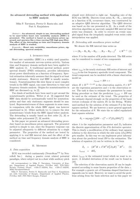
Abstract— <strong>An</strong> <strong>advanced</strong>, simple <strong>to</strong> use, <strong>detrending</strong> <strong>method</strong><br />
<strong>to</strong> be used before heart rate variability <strong>analysis</strong> (<strong>HRV</strong>) is<br />
presented. The <strong>method</strong> is based on smoothness priors approach<br />
and operates like a time-varying FIR high pass filter.<br />
The effect of the <strong>detrending</strong> on time and frequency domain<br />
<strong>analysis</strong> of <strong>HRV</strong> is studied.<br />
Keywords— Heart rate variability, smoothness priors, signal<br />
<strong>detrending</strong>, spectral <strong>analysis</strong>.<br />
I. Introduction<br />
Heart rate variability (<strong>HRV</strong>) is a widely used quantitative<br />
marker of au<strong>to</strong>nomic nervous system activity. Various<br />
time and frequency domain <strong>method</strong>s have been applied <strong>to</strong><br />
<strong>HRV</strong> <strong>analysis</strong> [1]. A traditional spectral <strong>method</strong>, power<br />
spectral density (PSD) estimation, provides information<br />
about power distribution as a function of frequency. Spectral<br />
estimation inherently assumes that the signal is at least<br />
weakly stationary. However real <strong>HRV</strong> is usually nonstationary.<br />
Nonstationarities like slow linear or more complex<br />
trends in the <strong>HRV</strong> signal, can cause dis<strong>to</strong>rtion <strong>to</strong> time and<br />
frequency domain <strong>analysis</strong>. Origins for nonstationarities in<br />
<strong>HRV</strong> are discussed e.g. in [2].<br />
Two kinds of <strong>method</strong>s have been used <strong>to</strong> get around the<br />
nonstationarity problem. Weber et al. [3] suggested that<br />
<strong>HRV</strong> data should be systematically tested for nonstationarities<br />
and that only stationary segments should be analyzed.<br />
Representativeness of these segments in some cases,<br />
in comparison <strong>with</strong> the whole <strong>HRV</strong> signal, was however<br />
questioned in [4]. Other <strong>method</strong>s try <strong>to</strong> remove the slow<br />
nonstationary trends from the <strong>HRV</strong> signal before <strong>analysis</strong>.<br />
The <strong>detrending</strong> is usually based on first order [5], [6] or<br />
higher order polynomial [7], [6] models.<br />
In this paper we present an <strong>advanced</strong> <strong>detrending</strong> procedure<br />
based on smoothness priors approach. The presented<br />
<strong>method</strong> is simple <strong>to</strong> use, since the frequency response can<br />
be adjusted adequately <strong>to</strong> different situations by a single<br />
parameter. The properties of the <strong>method</strong> are tested by<br />
applying it <strong>to</strong> real RR interval data and the effect of the<br />
<strong>method</strong> on time and frequency domain <strong>analysis</strong> of <strong>HRV</strong> is<br />
considered.<br />
A. Data acquisition<br />
II. Methods<br />
ECG was recorded continuously (NeuroScan TM by NeuroSoft<br />
Inc.) during a passive event related potential<br />
paradigm, where subject sat in a chair while audi<strong>to</strong>ry pitch<br />
All correspondence <strong>to</strong> Mika P. Tarvainen, University of Kuopio,<br />
Department of Applied Physics, P.O.Box 1627, FIN-70211<br />
Kuopio, Finland, Phone. +358-17-162584, Fax. +358-17-162585,<br />
Mika.Tarvainen@uku.fi<br />
Mika P. Tarvainen, Perttu O. Ranta-aho and Pasi A. Karjalainen<br />
are <strong>with</strong> University of Kuopio, Department of Applied Physics,<br />
P.O.Box 1627, FIN-70211 Kuopio, Finland<br />
stimuli were delivered <strong>to</strong> right ear. Sampling rate of the<br />
ECG was 500 Hz. Discrete event series, R i −R i−1 intervals<br />
as a function of R i occurrence times, was constructed by<br />
an adaptive QRS detec<strong>to</strong>r algorithm. The QRS detec<strong>to</strong>r<br />
was based on the one presented in [8]. As a result of the<br />
detection algorithm an unevenly sampled RR interval time<br />
series was obtained. In order <strong>to</strong> recover an evenly sampled<br />
signal from the irregularly sampled event series cubic<br />
interpolation was applied.<br />
B. Detrending <strong>with</strong> smoothness priors <strong>method</strong><br />
We denote the RR interval time series as<br />
z = (R 2 − R 1 ,R 3 − R 2 , . . . ,R N − R N−1 ) T ∈ R N−1 (1)<br />
where N is the number of R peaks detected. The RR series<br />
can be considered <strong>to</strong> consist of two components<br />
z = z stat + z trend (2)<br />
where z stat is the nearly stationary RR series of interest and<br />
z trend is the low frequency aperiodic trend component. The<br />
trend component can be modeled <strong>with</strong> a linear observation<br />
model as<br />
z trend = Hθ + v (3)<br />
where H ∈ R (N−1)×M is the observation matrix, θ ∈ R M<br />
are the regression parameters and v is the observation error.<br />
The task is then <strong>to</strong> estimate the parameters by some<br />
fitting procedure so that the prediction ẑ trend = Hˆθ can<br />
be used as the estimate of the trend. The properties of<br />
the estimate depend strongly on the properties of the basis<br />
vec<strong>to</strong>rs (columns of the matrix H) in the fitting. Widely<br />
used <strong>method</strong> for the solution of the estimate ˆθ is the least<br />
squares <strong>method</strong>. We use however a more general approach<br />
for the estimation of ˆθ. We state the so called regularized<br />
least squares solution<br />
ˆθ λ = arg min<br />
θ<br />
{<br />
‖Hθ − z‖ 2 + λ 2 ‖D d (Hθ)‖ 2} (4)<br />
where λ is the regularization parameter and D d indicates<br />
the discrete approximation of the d’th derivative opera<strong>to</strong>r.<br />
This is clearly a modification of the ordinary least squares<br />
solution <strong>to</strong> the direction in which the side norm ‖D d (Hθ)‖<br />
gets smaller. In this way we can implement prior information<br />
about the predicted trend Hθ <strong>to</strong> the estimation. The<br />
solution of equation (4) can be written in the form<br />
ˆθ λ = ( H T H + λ 2 H T D T d D d H ) −1<br />
H T z (5)<br />
ẑ trend = Hˆθ λ (6)<br />
where ẑ trend is the estimated trend which we want <strong>to</strong> remove.<br />
A detailed derivation of the result can be found in<br />
[10].<br />
The selection of the observation matrix H can be implemented<br />
according <strong>to</strong> some known properties of the data z.<br />
For example a generic set of Gaussian shaped functions or<br />
sigmoids can be used. However, we want <strong>to</strong> avoid the problems<br />
arising from the basis selection and in this paper we
2<br />
1<br />
Magnitude<br />
1<br />
0.5<br />
Magnitude<br />
0.5<br />
0.5 0<br />
0.25<br />
Normalized frequency<br />
0<br />
0<br />
10<br />
Discrete time<br />
20<br />
a) b)<br />
0<br />
0 0.1 0.2 0.3 0.4 0.5<br />
Normalized frequency<br />
Fig. 1. a) Time-varying frequency response of L (N − 1 = 50 and λ = 10). Only the first half of the frequency response is presented, since<br />
the other half is identical. b) Frequency responses, obtained from the middle row of L (cf. bold lines), for λ = 1, 2, 4, 10, 20, 50 and<br />
300. The corresponding cut-off frequencies are 0.189, 0.132, 0.093, 0.059, 0.041, 0.025 and 0.011 times the sampling frequency.<br />
use the trivial choice of identity matrix for the observation<br />
matrix H = I ∈ R (N−1)×(N−1) . The regularization part<br />
of (4) can be unders<strong>to</strong>od <strong>to</strong> draw the solution <strong>to</strong>wards the<br />
null space of the regularization matrix D d . The null space<br />
of the second order difference matrix contains all first order<br />
curves and thus D 2 is a good choice for estimating the<br />
aperiodic trend of RR series. The second order difference<br />
matrix D 2 ∈ R (N−3)×(N−1) is of the form<br />
⎛<br />
⎞<br />
1 −2 1 0 · · · 0<br />
.<br />
D 2 =<br />
0 1 −2 1 ..<br />
. ..<br />
⎜<br />
⎝<br />
.<br />
. .. . .. . .. . ⎟ .. 0 ⎠<br />
0 · · · 0 1 −2 1<br />
With these specific choices the <strong>method</strong> is called the smoothness<br />
priors <strong>method</strong> [11] and the detrended nearly stationary<br />
RR series can be written as<br />
(7)<br />
ẑ stat = z − Hˆθ λ = ( I − (I + λ 2 D T 2 D 2 ) −1) z (8)<br />
C. PSD estimation<br />
Methods for PSD estimation can be classified as nonparametric<br />
(e.g. <strong>method</strong>s based on FFT) and parametric<br />
(<strong>method</strong>s based on e.g. au<strong>to</strong>regressive (AR) time series<br />
modeling). In the latter approach the RR time series is<br />
modeled as an AR(p) process<br />
z t = −<br />
p∑<br />
a j z t−j + e t , t = p + 1, . . . , N − 1 (9)<br />
j=1<br />
where p is the model order, a j are the AR coefficients and<br />
e t is the noise term. A modified covariance <strong>method</strong> is used<br />
<strong>to</strong> solve the AR model. The power spectrum estimate P z<br />
is then calculated as<br />
P z (ω) =<br />
σ 2<br />
|1 + ∑ p<br />
j=1 a je −iωj | 2 (10)<br />
where σ 2 is the variance of the prediction error of the<br />
model. [12]<br />
III. Results<br />
In order <strong>to</strong> demonstrate the properties of the proposed<br />
<strong>detrending</strong> <strong>method</strong>, we first consider it’s frequency response.<br />
Equation (8) can be written as ẑ stat = Lz, where<br />
L = I − (I + λ 2 D T 2 D 2 ) −1 corresponds <strong>to</strong> a time-varying<br />
FIR high pass filter. The frequency response of L for each<br />
discrete time point, obtained as a Fourier transform of it’s<br />
rows, is presented in Fig. 1 a). It can be seen that the filter<br />
is mostly constant, but the beginning and end of the signal<br />
are handled differently. The filtering effect is attenuated<br />
for the first and last elements of z, and thus the dis<strong>to</strong>rtion<br />
of end points of data is avoided. The effect of the smoothing<br />
parameter λ on the frequency response of the filter is<br />
presented in Fig. 1 b). The cut-off frequency of the filter<br />
decreases when λ is increased. Besides the λ parameter the<br />
frequency response naturally depends on the sampling rate<br />
of signal z.<br />
The performance of the presented <strong>method</strong> on real RR interval<br />
time series data is presented in Fig. 2, where it is applied<br />
<strong>to</strong> RR data of four different subjects. Each RR series<br />
was first interpolated <strong>to</strong> obtain a regularly sampled series<br />
<strong>with</strong> sampling rate of 4 Hz. The <strong>detrending</strong> was then performed<br />
using a smoothing parameter λ = 300, which equals<br />
a cut-off frequency of 0.043 Hz. The four RR series <strong>with</strong><br />
the fitted trends and the corresponding detrended series are<br />
presented in Fig. 2 a). Three different time domain parameters,<br />
recommended in [1], were selected <strong>to</strong> demonstrate the<br />
effect of the used <strong>detrending</strong> <strong>method</strong> on time domain <strong>analysis</strong><br />
(Fig. 2 b)). These were the standard deviation of all<br />
RR intervals (SDNN), the square root of the mean squared<br />
differences of successive RR intervals (RMSSD) and the<br />
relative amount of successive RR intervals differing more<br />
than 50 ms (pNN50).<br />
The effect of the presented <strong>detrending</strong> <strong>method</strong> on<br />
the PSD estimates calculated <strong>with</strong> Welch’s periodogram<br />
<strong>method</strong> and by AR modeling is presented in Fig. 2 c). AR<br />
model order p = 16 was selected according <strong>to</strong> [1], by using<br />
the corrected Akaike information criteria [13]. In each<br />
original PSD estimate the intensity of the very low frequency<br />
(VLF) component is clearly stronger than the intensity<br />
of low frequency (LF) or high frequency (HF) com-
3<br />
a) Original and detrended RR series<br />
RRI (s)<br />
1.1<br />
0.9<br />
0.7<br />
0.2<br />
0<br />
−0.2<br />
0 100 200 0 100 200 0 100 200 0 100 200<br />
Time (s)<br />
b) Time domain <strong>analysis</strong><br />
SDNN RMSSD pNN50 SDNN RMSSD pNN50 SDNN RMSSD pNN50 SDNN RMSSD pNN50<br />
(ms) (ms) (%) (ms) (ms) (%) (ms) (ms) (%) (ms) (ms) (%)<br />
Original 63.62 72.40 53.00 60.96 37.34 16.80 53.01 62.72 53.95 52.93 37.48 17.29<br />
Detrended 55.54 72.10 52.07 41.42 36.98 15.98 49.15 62.51 54.42 41.90 37.21 16.92<br />
c) Frequency domain <strong>analysis</strong><br />
PSD (s 2 /Hz)<br />
0.03<br />
0.02<br />
0.01<br />
0<br />
0.03<br />
0.02<br />
0.01<br />
0<br />
0 0.25 0.5<br />
0 0.25 0.5 0 0.25 0.5 0 0.25 0.5<br />
Frequency (Hz)<br />
Fig. 2. The effect of the <strong>detrending</strong> <strong>method</strong> on time and frequency domain <strong>analysis</strong>. a) Original RR series and fitted trends (above) and<br />
detrended RR series (below) for four different data segments. The duration of each data segment is 200 seconds and they were obtained<br />
from different subjects. b) The effect of the <strong>detrending</strong> procedure on three time domain parameters (SDNN, RMSSD and pNN50). c)<br />
PSD estimates for original (thin line) and detrended (bold line) RR series <strong>with</strong> Welch’s periodogram <strong>method</strong> (above) and by using a<br />
16’th order AR model (below).<br />
ponent. Each spectrum is however limited <strong>to</strong> 0.035 s 2 /Hz<br />
<strong>to</strong> enable the comparison of the spectrums before and after<br />
<strong>detrending</strong>. For Welch’s <strong>method</strong> the VLF components are<br />
properly removed while the higher frequencies are not significantly<br />
altered by the <strong>detrending</strong>. But when AR models<br />
of relatively low orders are used, which is usually desirable<br />
in <strong>HRV</strong> <strong>analysis</strong> in order <strong>to</strong> enable a distinct division of<br />
the spectrum in<strong>to</strong> VLF, LF and HF components, the effect<br />
of <strong>detrending</strong> is remarkable. In each original AR spectrum<br />
the peak around 0.1 Hz is spuriously covered by the strong<br />
VLF component. However in the AR spectrums obtained<br />
after <strong>detrending</strong> the component near 0.1 Hz is more realistic<br />
when compared <strong>to</strong> the spectrums obtained by Welch’s<br />
<strong>method</strong>.<br />
IV. Discussion<br />
We have presented an <strong>advanced</strong> <strong>detrending</strong> <strong>method</strong> <strong>with</strong><br />
<strong>application</strong> <strong>to</strong> <strong>HRV</strong> <strong>analysis</strong>. The <strong>method</strong> is based on<br />
smoothness priors formulation. The main advantage of the<br />
<strong>method</strong>, compared <strong>to</strong> <strong>method</strong>s presented in [7], [5], is its<br />
simplicity. The frequency response of the <strong>method</strong> is adjusted<br />
<strong>with</strong> a single parameter. This smoothing parameter<br />
λ should be selected in such a way that the spectral<br />
components of interest are not significantly affected by the<br />
<strong>detrending</strong>. <strong>An</strong>other advantage of the presented <strong>method</strong> is<br />
that the filtering effect is attenuated in the beginning and<br />
the end of the data and thus the dis<strong>to</strong>rtion of data end<br />
points is avoided.<br />
The effect of <strong>detrending</strong> on time and frequency domain<br />
<strong>analysis</strong> of <strong>HRV</strong> was demonstrated. In time domain most<br />
effect is focused on SDNN, which describes the amount<br />
of overall variance of RR series. Instead only little effect<br />
is focused on RMSSD and pNN50 which both describe the<br />
differences in successive RR intervals. In frequency domain<br />
the low frequency trend components increase the power of<br />
VLF component. Thus, when using relatively low order<br />
AR models in spectrum estimation <strong>detrending</strong> is especially<br />
recommended, since the strong VLF component dis<strong>to</strong>rts<br />
other components, especially the LF component, of the<br />
spectrum.<br />
The presented <strong>detrending</strong> <strong>method</strong> can be applied <strong>to</strong> e.g.<br />
respira<strong>to</strong>ry sinus arrhythmia (RSA) quantification. RSA<br />
component is separated from other frequency components<br />
of <strong>HRV</strong> by adjusting the smoothing parameter λ properly.<br />
For other purposes of <strong>HRV</strong> <strong>analysis</strong> one should make sure<br />
that the <strong>detrending</strong> does not lose any useful information<br />
from the lower frequency components. Finally, it should<br />
be emphasized that the presented <strong>detrending</strong> <strong>method</strong> is<br />
not restricted <strong>to</strong> <strong>HRV</strong> <strong>analysis</strong> only, but can be applied as<br />
well <strong>to</strong> other biomedical signals e.g. for <strong>detrending</strong> of EEG<br />
signals in quantitative EEG <strong>analysis</strong>.
4<br />
Appendix<br />
All the computation of this paper are executed using<br />
MATLAB R 6 of The MathWorks Inc. The source code,<br />
in all its simplicity, for applying the presented <strong>detrending</strong><br />
<strong>method</strong> <strong>to</strong> signal z is listed below.<br />
T = length(z);<br />
lambda = 10;<br />
I = speye(T);<br />
D2 = spdiags(ones(T-2,1)*[1 -2 1],[0:2],T-2,T);<br />
z_stat = (I-inv(I+lambda^2*D2’*D2))*z;<br />
For more information see<br />
http://venda.uku.fi/research/biosignals<br />
References<br />
[1] Task force of the European society of cardiology and the North<br />
American society of pacing and electrophysiology, “Heart rate<br />
variability – standards of measurement, physiological interpretation,<br />
and clinical use,” Circulation, vol. 93, pp. 1043–1065,<br />
March 1996.<br />
[2] G. Berntson, J. B. JR., D. Eckberg, P. Grossman, P. Kaufmann,<br />
M. Malik, H. Nagaraja, S. Porges, J. Saul, P. S<strong>to</strong>ne, and<br />
W. V. D. Molen, “Heart rate variability: Origins, <strong>method</strong>s, and<br />
interpretive caveats,” Psychophysiol, vol. 34, pp. 623–648, 1997.<br />
[3] E. Weber, C. Molenaar, and M. van der Molen, “A nonstationarity<br />
test for the spectral <strong>analysis</strong> of physiological time series <strong>with</strong><br />
an <strong>application</strong> <strong>to</strong> respira<strong>to</strong>ry sinus arrhythmia,” Psychophysiol,<br />
vol. 29, pp. 55–65, January 1992.<br />
[4] P. Grossman, “Breathing rhythms of the heart in a world of<br />
no steady state: a comment on Weber, Molenaar, and van der<br />
Molen,” Psychophysiol, vol. 29, pp. 66–72, January 1992.<br />
[5] D. Litvack, T. Oberlander, L. Carney, and J. Saul, “Time and<br />
frequency domain <strong>method</strong>s for heart rate variability <strong>analysis</strong>: a<br />
<strong>method</strong>ological comparison,” Psychophysiol, vol. 32, pp. 492–<br />
504, 1995.<br />
[6] I. Mi<strong>to</strong>v, “A <strong>method</strong> for assessment and processing of biomedical<br />
signals containing trend and periodic components,” Med Eng<br />
Phys, vol. 20, pp. 660–668, November-December 1998.<br />
[7] S. Porges and R. Bohrer, “The <strong>analysis</strong> of periodic processes<br />
in psychophysiological research,” in Principles of psychophysiology:<br />
physical social and inferential elements (J. Cacioppo and<br />
L. Tassinary, eds.), pp. 708–753, Cambridge University Press,<br />
1990.<br />
[8] J. Pan and W. Tompkins, “A real-time QRS detection algorithm,”<br />
IEEE Trans Biomed Eng, vol. 32, pp. 230–236, March<br />
1985.<br />
[9] P. Grossman, J. van Beek, and C. Wientjes, “A comparison<br />
of three quantification <strong>method</strong>s for estimation of respira<strong>to</strong>ry sinus<br />
arrhythmia,” Psychophysiol, vol. 27, pp. 702–714, November<br />
1990.<br />
[10] P. Karjalainen, Regularization and Bayesian <strong>method</strong>s for<br />
evoked potential esimation. PhD thesis, University of<br />
Kuopio, Department of Applied Physics, 1997. URL:<br />
http://venda.uku.fi/research/biosignal/publications/.<br />
[11] W. Gersch, “Smoothness priors,” in New Directions in Time<br />
Series <strong>An</strong>alysis, Part II, pp. 113–146, Springer-Verlag, 1991.<br />
[12] S. Marple, Digital Spectral <strong>An</strong>alysis <strong>with</strong> Applications. Prentice-<br />
Hall, 1987.<br />
[13] F. Gustafsson and H. Hjalmarsson, “Twenty-one ML estima<strong>to</strong>rs<br />
for model selection,” Au<strong>to</strong>matica, vol. 31, pp. 1377–1392, 1995.