Sample Size Calculations for Analytic Studies
Sample Size Calculations for Analytic Studies
Sample Size Calculations for Analytic Studies
Create successful ePaper yourself
Turn your PDF publications into a flip-book with our unique Google optimized e-Paper software.
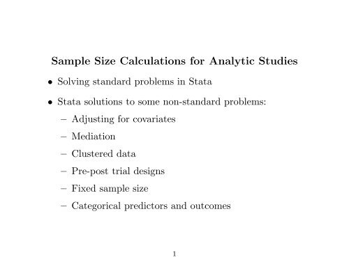
<strong>Sample</strong> <strong>Size</strong> <strong>Calculations</strong> <strong>for</strong> <strong>Analytic</strong> <strong>Studies</strong><br />
• Solving standard problems in Stata<br />
• Stata solutions to some non-standard problems:<br />
– Adjusting <strong>for</strong> covariates<br />
– Mediation<br />
– Clustered data<br />
– Pre-post trial designs<br />
– Fixed sample size<br />
– Categorical predictors and outcomes<br />
1
Standard problems<br />
• Method <strong>for</strong> calculating sample size depends on<br />
– Predictor type: continuous, binary<br />
– Outcome type: continuous, binary, failure time<br />
– Effect size<br />
– α, 1- or 2-sided test, power<br />
2
Binary predictor, continuous outcomes<br />
• Predictor prevalence 0.5 (e.g., RCTs with 1-1 allocation):<br />
– use Table 6.A. <strong>for</strong> comparing means in Designing<br />
Clinical Research (DCR)<br />
• Arbitrary predictor prevalence:<br />
– use sampsi function in Stata<br />
3
Basic set-up using sampsi<br />
Equal allocation to groups, means of 1.4 and 1.9, SD of<br />
outcome = 2 in both groups<br />
. sampsi 1.4 1.9, sd1(2)<br />
Estimated sample size <strong>for</strong> two-sample comparison of means<br />
Test Ho: m1 = m2, where m1 is the mean in population 1<br />
and m2 is the mean in population 2<br />
Assumptions:<br />
alpha = 0.0500 (two-sided)<br />
power = 0.9000<br />
m1 = 1.4<br />
m2 = 1.9<br />
sd1 = 2<br />
sd2 = 2<br />
n2/n1 = 1.00<br />
Estimated required sample sizes:<br />
n1 = 337<br />
n2 = 337<br />
4
A more complicated example<br />
60% in group 2, means 1.4 and 1.6, SDs of 0.85 and 1.05,<br />
one-sided test<br />
. local r = .6/.4<br />
. sampsi 1.4 1.6, sd1(0.85) sd2(1.05) r(‘r’) power(0.8) onesided<br />
Estimated sample size <strong>for</strong> two-sample comparison of means<br />
Test Ho: m1 = m2, where m1 is the mean in population 1<br />
and m2 is the mean in population 2<br />
Assumptions:<br />
alpha = 0.0500 (one-sided)<br />
power = 0.8000<br />
m1 = 1.4<br />
m2 = 1.6<br />
sd1 = .85<br />
sd2 = 1.05<br />
n2/n1 = 1.50<br />
Estimated required sample sizes:<br />
n1 = 226<br />
n2 = 339<br />
Note: Use sampncti <strong>for</strong> large effect sizes; requires nct2 package<br />
5
Continuous predictor, continuous outcome<br />
• If you can pose problem in terms of correlation coefficient:<br />
– use Table 6.C <strong>for</strong> in DCR<br />
– use sampsi rho in STATA<br />
• If you can pose problem in terms of slope, SDs of<br />
predictor and outcome:<br />
– use sampsi reg<br />
6
Continuous predictor, continuous outcome,<br />
using sampsi rho<br />
Correlation of predictor and outcome = 0.3<br />
. sampsi_rho, alt(0.3) power(0.8)<br />
Estimated sample size <strong>for</strong> Pearson Correlation<br />
Test Ho: Rho alt = Rho null, usually null Rho is 0<br />
Assumptions:<br />
Alpha = 0.0500 (two-sided)<br />
Power = 0.8000<br />
Null Rho = 0.0000<br />
Alt Rho = 0.3000<br />
Estimated required sample size:<br />
n = 84.927811<br />
7
Continuous predictor, continuous outcome,<br />
using sampsi reg<br />
Regression coefficient = 0.3, SD of predictor and outcome = 1<br />
. sampsi_reg, alt(0.3) sx(1) sy(1) varmethod(sdy) power(0.8)<br />
Estimated sample size <strong>for</strong> linear regression<br />
Test Ho: slope alt = slope null, usually null slope is 0<br />
Assumptions:<br />
Alpha = 0.0500 (two-sided)<br />
Power = 0.8000<br />
Null Slope = 0.0000<br />
Alt Slope = 0.3000<br />
Residual sd = 0.9539<br />
SD of X’s = 1.0000<br />
SD of Y’s = 1.0000<br />
Estimated required sample size:<br />
n = 82<br />
8
Binary predictor, binary outcome<br />
• Predictor prevalence 0.5<br />
– use Table 6.B. <strong>for</strong> comparing proportions in DCR<br />
• Arbitrary predictor prevalence:<br />
– use sampsi function in Stata<br />
9
Binary predictor, binary outcome<br />
Exposure prevalence 2/3, outcome prevalence 20% in<br />
unexposed, 30% in exposed<br />
. sampsi 0.2 0.3, r(2) power(0.8)<br />
Estimated sample size <strong>for</strong> two-sample comparison of proportions<br />
Test Ho: p1 = p2, where p1 is the proportion in population 1<br />
and p2 is the proportion in population 2<br />
Assumptions:<br />
alpha = 0.0500 (two-sided)<br />
power = 0.8000<br />
p1 = 0.2000<br />
p2 = 0.3000<br />
n2/n1 = 2.00<br />
Estimated required sample sizes:<br />
n1 = 239<br />
n2 = 478<br />
10
Continuous predictor, binary outcome<br />
• Use methods <strong>for</strong> binary predictor, continuous outcome<br />
– set r = p/(1 − p) where p is prevalence of outcome<br />
– if you know means and SDs of continuous predictor in<br />
cases and controls, use sampsi as usual<br />
– otherwise, set up using log-OR and SD of predictor<br />
11
Continuous predictor, binary outcome<br />
Case-control study with 3 controls per case, mean of<br />
predictor 0.2 in controls, 0.4 in cases, SD of predictor 0.5 in<br />
both groups<br />
. sampsi 0.2 0.4, r(.33) sd1(0.5)<br />
Estimated sample size <strong>for</strong> two-sample comparison of means<br />
Test Ho: m1 = m2, where m1 is the mean in population 1<br />
and m2 is the mean in population 2<br />
Assumptions:<br />
alpha = 0.0500 (two-sided)<br />
power = 0.9000<br />
m1 = .2<br />
m2 = .4<br />
sd1 = .5<br />
sd2 = .5<br />
n2/n1 = 0.33<br />
Estimated required sample sizes:<br />
n1 = 265<br />
n2 = 88<br />
12
Continuous predictor, binary outcome<br />
Cross-sectional study with outcome prevalence = 33%, OR<br />
per unit increase in predictor = 1.5, SD of predictor = 0.5:<br />
effect size equal to log(OR) × SD of predictor<br />
. local delta = log(1.5)*0.5<br />
. sampsi 0 ‘delta’, r(0.5) sd1(1) power(0.8)<br />
Estimated sample size <strong>for</strong> two-sample comparison of means<br />
Test Ho: m1 = m2, where m1 is the mean in population 1<br />
and m2 is the mean in population 2<br />
Assumptions:<br />
alpha = 0.0500 (two-sided)<br />
power = 0.8000<br />
m1 = 0<br />
m2 = .202733<br />
sd1 = 1<br />
sd2 = 1<br />
n2/n1 = 0.50<br />
Estimated required sample sizes:<br />
n1 = 573<br />
n2 = 287<br />
13
Failure time outcomes<br />
• Use stpower in STATA<br />
– stpower cox <strong>for</strong> Cox models<br />
– stpower logrank <strong>for</strong> unadjusted log-rank test<br />
– stpower exponential <strong>for</strong> trials with long accrual<br />
14
Continuous predictor, failure time outcome<br />
Overall cumulative incidence of 15%, 10% early dropout, SD<br />
of predictor 1.5, hazard-ratio per unit increase in predictor 1.2<br />
. stpower cox, failprob(0.15) wdprob(0.10) sd(1.5) hratio(1.2)<br />
Estimated sample size <strong>for</strong> Cox PH regression<br />
Wald test, log-hazard metric<br />
Ho: [b1, b2, ..., bp] = [0, b2, ..., bp]<br />
Input parameters:<br />
alpha = 0.0500 (two sided)<br />
b1 = 0.1823<br />
sd = 1.5000<br />
power = 0.8000<br />
Pr(event) = 0.1500<br />
withdrawal(%) = 10.00<br />
Estimated number of events and sample size:<br />
E = 105<br />
N = 778<br />
15
Binary predictor, failure time outcome<br />
RCT, overall cumulative incidence of 15%, 10% early<br />
dropout, hazard-ratio <strong>for</strong> treatment = 0.75, 1-1 allocation so<br />
SD of predictor = √ 0.5(1 − 0.5) = 0.5 (the default)<br />
. stpower cox, failprob(0.15) wdprob(0.10) hratio(0.75)<br />
Estimated sample size <strong>for</strong> Cox PH regression<br />
Wald test, log-hazard metric<br />
Ho: [b1, b2, ..., bp] = [0, b2, ..., bp]<br />
Input parameters:<br />
alpha = 0.0500 (two sided)<br />
b1 = -0.2877<br />
sd = 0.5000<br />
power = 0.8000<br />
Pr(event) = 0.1500<br />
withdrawal(%) = 10.00<br />
Estimated number of events and sample size:<br />
E = 380<br />
N = 2811<br />
16
Binary predictor, failure time outcome<br />
Overall cumulative incidence of 15%, 10% early dropout,<br />
prevalence of exposure 25%, hazard-ratio <strong>for</strong> exposure 1.5<br />
. local sd = sqrt(0.25*(1-0.25))<br />
. stpower cox, failprob(0.15) wdprob(0.10) hratio(1.50) sd(‘sd’)<br />
Estimated sample size <strong>for</strong> Cox PH regression<br />
Wald test, log-hazard metric<br />
Ho: [b1, b2, ..., bp] = [0, b2, ..., bp]<br />
Input parameters:<br />
alpha = 0.0500 (two sided)<br />
b1 = 0.4055<br />
sd = 0.4330<br />
power = 0.8000<br />
Pr(event) = 0.1500<br />
withdrawal(%) = 10.00<br />
Estimated number of events and sample size:<br />
E = 255<br />
N = 1887<br />
17
Adjustment <strong>for</strong> covariates<br />
• Suppose that<br />
– multiple correlation of primary predictor with<br />
covariates is ρ<br />
– equivalently R 2 <strong>for</strong> linear regression of primary<br />
predictor on covariates is ρ 2<br />
• Implemented in stpower using r2() option<br />
• Alternatively, compute sample size using sampsi, inflate<br />
result by 1/(1 − ρ 2 )<br />
• Hsieh recommends ρ = 0.3 → 10% inflation of N<br />
• NB: Adjusted effect size usually smaller than unadjusted<br />
18
Binary predictor, failure time outcome<br />
Same problem as be<strong>for</strong>e; correlation of exposure with<br />
covariates ρ = 0.5, so R 2 = 0.5 2 = 0.25<br />
. local sd = sqrt(0.25*(1-0.25))<br />
. stpower cox, failprob(0.15) wdprob(0.10) hratio(1.50) sd(‘sd’) r2(0.25)<br />
Estimated sample size <strong>for</strong> Cox PH regression<br />
Wald test, log-hazard metric<br />
Ho: [b1, b2, ..., bp] = [0, b2, ..., bp]<br />
Input parameters:<br />
alpha = 0.0500 (two sided)<br />
b1 = 0.4055<br />
sd = 0.4330<br />
power = 0.8000<br />
Pr(event) = 0.1500<br />
R2 = 0.2500<br />
withdrawal(%) = 10.00<br />
Estimated number of events and sample size:<br />
E = 340<br />
N = 2515<br />
19
Adjustment <strong>for</strong> covariates:<br />
binary predictor, continuous outcome<br />
Prevalence of exposure 40%, Effect size 0.25, ρ = 0.3<br />
. local r = 0.4/0.6<br />
. sampsi 0 0.25, sd1(1) r(‘r’) power(0.8)<br />
Estimated sample size <strong>for</strong> two-sample comparison of means<br />
Test Ho: m1 = m2, where m1 is the mean in population 1<br />
and m2 is the mean in population 2<br />
Assumptions:<br />
alpha = 0.0500 (two-sided)<br />
power = 0.8000<br />
m1 = 0<br />
m2 = .25<br />
sd1 = 1<br />
sd2 = 1<br />
n2/n1 = 0.67<br />
Estimated required sample sizes:<br />
n1 = 314<br />
n2 = 210<br />
. dis round((314+210)/(1-0.3^2))<br />
576<br />
20
<strong>Sample</strong> size to show mediation<br />
• To show mediation, we need to show that<br />
1. primary predictor associated with mediator<br />
2. mediator independently associated with outcome,<br />
adjusting <strong>for</strong> primary predictor<br />
3. coefficient <strong>for</strong> primary predictor changes when<br />
mediator added to the regression model<br />
• If 1 holds, then 2 implies 3<br />
• Determine sample size needed to show 2:<br />
– mediator independently predicts outcome, adjusting<br />
<strong>for</strong> primary predictor and covariates<br />
21
Mediation example<br />
Cox model, cumulative incidence 25%, early dropout 15%,<br />
adjusted HR per SD increase in continuous mediator 1.2,<br />
correlation of mediator w/ primary predictor, covariates 0.2<br />
. stpower cox, failprob(0.25) wdprob(0.15) hratio(1.2) sd(1) r2(0.04)<br />
Estimated sample size <strong>for</strong> Cox PH regression<br />
Wald test, log-hazard metric<br />
Ho: [b1, b2, ..., bp] = [0, b2, ..., bp]<br />
Input parameters:<br />
alpha = 0.0500 (two sided)<br />
b1 = 0.1823<br />
sd = 1.0000<br />
power = 0.8000<br />
Pr(event) = 0.2500<br />
R2 = 0.0400<br />
withdrawal(%) = 15.00<br />
Estimated number of events and sample size:<br />
E = 246<br />
N = 1158<br />
22
Cluster randomized trials<br />
• Clusters of average size n c are randomized 1-1 to<br />
treatment or control<br />
• Compute number of patients <strong>for</strong> trial ignoring clustering<br />
• Inflate N by “design effect”: 1 + ρ(n c − 1), where ρ is the<br />
within-cluster correlation<br />
• sampclus implements this after sampsi (but not<br />
stpower)<br />
23
Cluster randomized trials<br />
Binary outcome, incidence 30% in control, 20% in treatment,<br />
1-1 allocation of clusters, n c = 25, ρ = 0.02<br />
. sampsi 0.3 0.2<br />
Estimated sample size <strong>for</strong> two-sample comparison of proportions<br />
Test Ho: p1 = p2, where p1 is the proportion in population 1<br />
and p2 is the proportion in population 2<br />
Assumptions:<br />
alpha = 0.0500 (two-sided)<br />
power = 0.9000<br />
p1 = 0.3000<br />
p2 = 0.2000<br />
n2/n1 = 1.00<br />
Estimated required sample sizes:<br />
n1 = 412<br />
n2 = 412<br />
. dis round(412*(1+0.02*24))<br />
610<br />
24
. sampclus, obsclus(25) rho(0.02)<br />
Cluster randomized trials<br />
<strong>Sample</strong> <strong>Size</strong> Adjusted <strong>for</strong> Cluster Design<br />
n1 (uncorrected) = 412<br />
n2 (uncorrected) = 412<br />
Intraclass correlation = .02<br />
Average obs. per cluster = 25<br />
Minimum number of clusters = 49<br />
Estimated sample size per group:<br />
n1 (corrected) = 610<br />
n2 (corrected) = 610<br />
25
Randomized trials, within-cluster randomization<br />
• Patients are randomized 1-1 to treatment or control<br />
within clusters<br />
• Design effect is 1 − ρ, does not depend on n c<br />
• Compute sample size ignoring clustering, multiply result<br />
by 1 − ρ<br />
26
Clustered data: complex surveys<br />
• Design effects vary by predictor and outcome, can be less<br />
than 1<br />
• Simple rules do not apply<br />
• Use design effect to adjust sample size calculated<br />
assuming independence, if you can get a reasonable<br />
estimate<br />
27
RCTs measuring change in a continuous outcome<br />
• Outcome measured at baseline and follow-up<br />
• No expected difference in means at baseline (why?)<br />
• Analysis options<br />
– analyze follow-up outcome, ignoring baseline<br />
– analyze change scores<br />
– analyze follow-up outcome, adjusting <strong>for</strong> baseline<br />
(ANCOVA)<br />
• Use sampsi<br />
28
RCT measuring change in continuous outcome<br />
1-1 allocation, equal baseline means, effect size at follow-up<br />
0.5 SD, correlation of baseline and follow-up outcome 0.3<br />
. sampsi 0 0.5, sd1(1) pre(1) post(1) r01(.3)<br />
Estimated sample size <strong>for</strong> two samples with repeated measures<br />
Assumptions:<br />
alpha = 0.0500 (two-sided)<br />
power = 0.9000<br />
m1 = 0<br />
m2 = .5<br />
sd1 = 1<br />
sd2 = 1<br />
n2/n1 = 1.00<br />
number of follow-up measurements = 1<br />
number of baseline measurements = 1<br />
correlation between baseline & follow-up = 0.300<br />
29
RCT measuring change in continuous outcome<br />
Method: POST<br />
relative efficiency = 1.000<br />
adjustment to sd = 1.000<br />
adjusted sd1 = 1.000<br />
Estimated required sample sizes:<br />
n1 = 85<br />
n2 = 85<br />
Method: CHANGE<br />
relative efficiency = 0.714<br />
adjustment to sd = 1.183<br />
adjusted sd1 = 1.183<br />
Estimated required sample sizes:<br />
n1 = 118<br />
n2 = 118<br />
Method: ANCOVA<br />
relative efficiency = 1.099<br />
adjustment to sd = 0.954<br />
adjusted sd1 = 0.954<br />
Estimated required sample sizes:<br />
n1 = 77<br />
n2 = 77<br />
30
Same design, but with pre-post correlation of 0.7<br />
Method: POST<br />
relative efficiency = 1.000<br />
adjustment to sd = 1.000<br />
adjusted sd1 = 1.000<br />
Estimated required sample sizes:<br />
n1 = 85<br />
n2 = 85<br />
Method: CHANGE<br />
relative efficiency = 1.667<br />
adjustment to sd = 0.775<br />
adjusted sd1 = 0.775<br />
Estimated required sample sizes:<br />
n1 = 51<br />
n2 = 51<br />
Method: ANCOVA<br />
relative efficiency = 1.961<br />
adjustment to sd = 0.714<br />
adjusted sd1 = 0.714<br />
Estimated required sample sizes:<br />
n1 = 43<br />
n2 = 43<br />
31
If sample size is fixed<br />
• In secondary analyses, sample size usually a done deal<br />
• sampsi can compute power <strong>for</strong> fixed N and effect size<br />
• stpower can compute either power or minimum<br />
detectable effects when other inputs are specified<br />
• In grants, power <strong>for</strong> a well-motivated effect size more<br />
convincing than minimum detectable effects<br />
32
Power <strong>for</strong> fixed sample and effect sizes<br />
Cox model, N=2515, 15% overall cumulative incidence, 10%<br />
dropout, 25% exposed, HR <strong>for</strong> exposure 1.5<br />
. local sd = sqrt(0.25*(1-0.25))<br />
. local n = round(2515*0.9)<br />
. stpower cox, failprob(0.15) hratio(1.3(0.1)1.6) sd(‘sd’) r2(0.25) n(‘n’)<br />
Estimated power <strong>for</strong> Cox PH regression<br />
Wald test, log-hazard metric<br />
Ho: [b1, b2, ..., bp] = [0, b2, ..., bp]<br />
+------------------------------------------------------------------------+<br />
| Power N E B1 SD Alpha* Pr(E) R2 |<br />
|------------------------------------------------------------------------|<br />
| .441616 2264 340 .262364 .433013 .05 .15 .25 |<br />
| .64254 2264 340 .336472 .433013 .05 .15 .25 |<br />
| .800117 2264 340 .405465 .433013 .05 .15 .25 |<br />
| .901134 2264 340 .470004 .433013 .05 .15 .25 |<br />
+------------------------------------------------------------------------+<br />
33
Minimum detectable hazard ratios<br />
Same set-up as last slide<br />
. local sd = sqrt(0.25*(1-0.25))<br />
. local n = round(2515*0.9)<br />
. stpower cox, failprob(0.15) sd(‘sd’) r2(0.25) n(‘n’) power(0.9) hr<br />
Estimated hazard ratio <strong>for</strong> Cox PH regression<br />
Wald test, hazard metric<br />
Ho: [b1, b2, ..., bp] = [0, b2, ..., bp]<br />
Input parameters:<br />
alpha = 0.0500 (two sided)<br />
sd = 0.4330<br />
N = 2264<br />
power = 0.9000<br />
Pr(event) = 0.1500<br />
R2 = 0.2500<br />
Estimated number of events and hazard ratio:<br />
E = 340<br />
hratio = 0.6256<br />
. dis 1/.6256<br />
1.5984655<br />
34
Categorical predictors and outcomes<br />
• Categorical predictors:<br />
– compute Ns <strong>for</strong> pairwise differences with reference<br />
group (multiple comparisons)<br />
– <strong>for</strong> overall effect, use fpower or simpower functions in<br />
STATA<br />
http://www.ats.ucla.edu/stat/stata/dae/fpower.htm<br />
• Categorical outcomes<br />
– nominal outcomes: compute Ns <strong>for</strong> pairwise<br />
differences with reference group<br />
– ordinal outcomes: Whitehead paper gives methods<br />
available <strong>for</strong> proportional odds model, but n/a in<br />
Stata<br />
35
Summary<br />
• Stata sampsi and stpower commands can do a lot,<br />
including making tables<br />
• stpower can account <strong>for</strong> covariate adjustment; with<br />
sampsi inflate sample size by 1/(1 − ρ 2 )<br />
• Handle mediation like a confounding problem<br />
• sampclus can inflate sample size <strong>for</strong> cluster-randomized<br />
trials with continuous or binary endpoint; <strong>for</strong> Cox model,<br />
inflate sample size by design effect 1 + ρ(n c − 1)<br />
• sampsi can handle simple pre-post designs<br />
• Downloadable Stata packages (and your biostat mentors)<br />
can deal with more complicated problems<br />
36


