- Page 1 and 2: Combining Pattern Classifiers
- Page 3 and 4: Copyright # 2004 by John Wiley & So
- Page 5 and 6: vi CONTENTS 1.5.2 Normal Distributi
- Page 7 and 8: viii CONTENTS 5.1.2 Probabilities B
- Page 9 and 10: x CONTENTS 9.1.1 Equivalence of MIN
- Page 11 and 12: Preface Everyday life throws at us
- Page 13 and 14: PREFACE xv employing it for buildin
- Page 15 and 16: Notation and Acronyms CART LDC MCS
- Page 17 and 18: 1 Fundamentals of Pattern Recogniti
- Page 19 and 20: BASIC CONCEPTS: CLASS, FEATURE, AND
- Page 21 and 22: CLASSIFIER, DISCRIMINANT FUNCTIONS,
- Page 23 and 24: CLASSIFIER, DISCRIMINANT FUNCTIONS,
- Page 25 and 26: CLASSIFICATION ERROR AND CLASSIFICA
- Page 27 and 28: CLASSIFICATION ERROR AND CLASSIFICA
- Page 29 and 30: EXPERIMENTAL COMPARISON OF CLASSIFI
- Page 31 and 32: EXPERIMENTAL COMPARISON OF CLASSIFI
- Page 33 and 34: EXPERIMENTAL COMPARISON OF CLASSIFI
- Page 35 and 36: EXPERIMENTAL COMPARISON OF CLASSIFI
- Page 37 and 38: EXPERIMENTAL COMPARISON OF CLASSIFI
- Page 39 and 40: EXPERIMENTAL COMPARISON OF CLASSIFI
- Page 41 and 42: BAYES DECISION THEORY 25 4. Make su
- Page 43 and 44: BAYES DECISION THEORY 27 Fig. 1.8 N
- Page 45 and 46: BAYES DECISION THEORY 29 coming fro
- Page 47 and 48: BAYES DECISION THEORY 31 because th
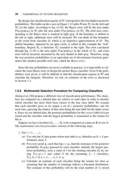
- Page 49: BAYES DECISION THEORY 33 The error
- Page 53 and 54: Holmström et al. [32] consider ano
- Page 55 and 56: K-HOLD-OUT PAIRED t-TEST 39 Fig. 1.
- Page 57 and 58: 5 2cv PAIRED t-TEST 41 for i=1:K l
- Page 59 and 60: DATA GENERATION: LISSAJOUS FIGURE D
- Page 61 and 62: 46 BASE CLASSIFIERS where P(v i ) i
- Page 63 and 64: 48 BASE CLASSIFIERS For the common
- Page 65 and 66: 50 BASE CLASSIFIERS error was 42.8
- Page 67 and 68: 52 BASE CLASSIFIERS Fig. 2.2 Classi
- Page 69 and 70: 54 BASE CLASSIFIERS 2.2.2 Parzen Cl
- Page 71 and 72: 56 BASE CLASSIFIERS 2.3 THE k-NEARE
- Page 73 and 74: 58 BASE CLASSIFIERS Fig. 2.4 Illust
- Page 75 and 76: 60 BASE CLASSIFIERS set are called
- Page 77 and 78: 62 BASE CLASSIFIERS TABLE 2.2 Error
- Page 79 and 80: 64 BASE CLASSIFIERS justification.
- Page 81 and 82: 66 BASE CLASSIFIERS Fig. 2.7 Illust
- Page 83 and 84: 68 BASE CLASSIFIERS For a ¼ 0 and
- Page 85 and 86: 70 BASE CLASSIFIERS Fig. 2.8 (a) An
- Page 87 and 88: 72 BASE CLASSIFIERS 2.4.2.3 Misclas
- Page 89 and 90: 74 BASE CLASSIFIERS 2.4.3 Stopping
- Page 91 and 92: 76 BASE CLASSIFIERS TABLE 2.4 A Tab
- Page 93 and 94: 78 BASE CLASSIFIERS then calculate
- Page 95 and 96: 80 BASE CLASSIFIERS pay off. Method
- Page 97 and 98: 82 BASE CLASSIFIERS mation involved
- Page 99 and 100: 84 BASE CLASSIFIERS . The threshold
- Page 101 and 102:
86 BASE CLASSIFIERS Fig. 2.16 (a) U
- Page 103 and 104:
88 BASE CLASSIFIERS Fig. 2.18 Possi
- Page 105 and 106:
90 BASE CLASSIFIERS Eq. (2.90) or E
- Page 107 and 108:
92 BASE CLASSIFIERS of E (the updat
- Page 109 and 110:
94 BASE CLASSIFIERS For input-to-hi
- Page 111 and 112:
96 BASE CLASSIFIERS chi2=tree_chi2(
- Page 113 and 114:
98 BASE CLASSIFIERS ind=1; leaf=0;
- Page 115 and 116:
100 BASE CLASSIFIERS % outputs of t
- Page 117 and 118:
102 MULTIPLE CLASSIFIER SYSTEMS Fig
- Page 119 and 120:
104 MULTIPLE CLASSIFIER SYSTEMS Fig
- Page 121 and 122:
106 MULTIPLE CLASSIFIER SYSTEMS is
- Page 123 and 124:
108 MULTIPLE CLASSIFIER SYSTEMS . u
- Page 125 and 126:
110 MULTIPLE CLASSIFIER SYSTEMS Rus
- Page 127 and 128:
112 FUSION OF LABEL OUTPUTS general
- Page 129 and 130:
114 FUSION OF LABEL OUTPUTS TABLE 4
- Page 131 and 132:
116 FUSION OF LABEL OUTPUTS and U m
- Page 133 and 134:
118 FUSION OF LABEL OUTPUTS TABLE 4
- Page 135 and 136:
120 FUSION OF LABEL OUTPUTS To rela
- Page 137 and 138:
122 FUSION OF LABEL OUTPUTS where j
- Page 139 and 140:
124 FUSION OF LABEL OUTPUTS Assigni
- Page 141 and 142:
126 FUSION OF LABEL OUTPUTS 4.4 NAI
- Page 143 and 144:
128 FUSION OF LABEL OUTPUTS s 2 ¼
- Page 145 and 146:
130 FUSION OF LABEL OUTPUTS CI(v j
- Page 147 and 148:
132 FUSION OF LABEL OUTPUTS first-o
- Page 149 and 150:
134 FUSION OF LABEL OUTPUTS The mut
- Page 151 and 152:
136 FUSION OF LABEL OUTPUTS Constru
- Page 153 and 154:
138 FUSION OF LABEL OUTPUTS TABLE 4
- Page 155 and 156:
140 FUSION OF LABEL OUTPUTS To labe
- Page 157 and 158:
142 FUSION OF LABEL OUTPUTS Fig. 4.
- Page 159 and 160:
144 FUSION OF LABEL OUTPUTS Next we
- Page 161 and 162:
146 FUSION OF LABEL OUTPUTS 3. None
- Page 163 and 164:
148 FUSION OF LABEL OUTPUTS Similar
- Page 165 and 166:
5 Fusion of Continuous- Valued Outp
- Page 167 and 168:
HOW DO WE GET PROBABILITY OUTPUTS?
- Page 169 and 170:
HOW DO WE GET PROBABILITY OUTPUTS?
- Page 171 and 172:
CLASS-CONSCIOUS COMBINERS 157 As se
- Page 173 and 174:
CLASS-CONSCIOUS COMBINERS 159 Fig.
- Page 175 and 176:
CLASS-CONSCIOUS COMBINERS 161 Fig.
- Page 177 and 178:
CLASS-CONSCIOUS COMBINERS 163 The c
- Page 179 and 180:
The mean of the error of D 1 is 0:2
- Page 181 and 182:
CLASS-CONSCIOUS COMBINERS 167 befor
- Page 183 and 184:
CLASS-CONSCIOUS COMBINERS 169 The f
- Page 185 and 186:
CLASS-INDIFFERENT COMBINERS 171 par
- Page 187 and 188:
CLASS-INDIFFERENT COMBINERS 173 The
- Page 189 and 190:
CLASS-INDIFFERENT COMBINERS 175 the
- Page 191 and 192:
WHERE DO THE SIMPLE COMBINERS COME
- Page 193 and 194:
WHERE DO THE SIMPLE COMBINERS COME
- Page 195 and 196:
WHERE DO THE SIMPLE COMBINERS COME
- Page 197 and 198:
WHERE DO THE SIMPLE COMBINERS COME
- Page 199 and 200:
WHERE DO THE SIMPLE COMBINERS COME
- Page 201 and 202:
COMMENTS 187 and the weighted produ
- Page 203 and 204:
6 Classifier Selection 6.1 PRELIMIN
- Page 205 and 206:
WHY CLASSIFIER SELECTION WORKS 191
- Page 207 and 208:
ESTIMATING LOCAL COMPETENCE DYNAMIC
- Page 209 and 210:
ESTIMATING LOCAL COMPETENCE DYNAMIC
- Page 211 and 212:
PREESTIMATION OF THE COMPETENCE REG
- Page 213 and 214:
SELECTION OR FUSION? 199 TABLE 6.2
- Page 215 and 216:
BASE CLASSIFIERS AND MIXTURE OF EXP
- Page 217 and 218:
7 Bagging and Boosting 7.1 BAGGING
- Page 219 and 220:
BAGGING 205 Since there are only tw
- Page 221 and 222:
BAGGING 207 and d j,1 (x) ¼ d j,2
- Page 223 and 224:
BAGGING 209 5. Repeat steps (1) to
- Page 225 and 226:
BAGGING 211 Fig. 7.4 Error rates fo
- Page 227 and 228:
BOOSTING 213 HEDGE (b) Given: D¼f
- Page 229 and 230:
BOOSTING 215 shows how the probabil
- Page 231 and 232:
BOOSTING 217 Fig. 7.8 Testing error
- Page 233 and 234:
BOOSTING 219 into account by the cl
- Page 235 and 236:
BOOSTING 221 Fig. 7.10 example. Mar
- Page 237 and 238:
BIAS-VARIANCE DECOMPOSITION 223 7.3
- Page 239 and 240:
BIAS-VARIANCE DECOMPOSITION 225 the
- Page 241 and 242:
BIAS-VARIANCE DECOMPOSITION 227 dis
- Page 243 and 244:
WHICH IS BETTER: BAGGING OR BOOSTIN
- Page 245 and 246:
PROOF OF THE ERROR FOR AdaBoost (TW
- Page 247 and 248:
PROOF OF THE ERROR FOR AdaBoost (TW
- Page 249 and 250:
PROOF OF THE ERROR FOR AdaBoost (C
- Page 251 and 252:
238 MISCELLANEA for tree classifier
- Page 253 and 254:
240 MISCELLANEA This greedy algorit
- Page 255 and 256:
242 MISCELLANEA better than the fit
- Page 257 and 258:
244 MISCELLANEA 8.2 ERROR CORRECTIN
- Page 259 and 260:
246 MISCELLANEA Exhaustive Codes. D
- Page 261 and 262:
248 MISCELLANEA Fig. 8.2 Three impl
- Page 263 and 264:
250 MISCELLANEA TABLE 8.3 Possible
- Page 265 and 266:
252 MISCELLANEA to be the sum of al
- Page 267 and 268:
254 MISCELLANEA 8.3.1.3 Jaccard Ind
- Page 269 and 270:
256 MISCELLANEA tive definition of
- Page 271 and 272:
258 MISCELLANEA . Randomizing. Some
- Page 273 and 274:
260 MISCELLANEA Fig. 8.7 Stacked cl
- Page 275 and 276:
262 MISCELLANEA The generic cluster
- Page 277 and 278:
264 MISCELLANEA The ultimate goal o
- Page 279 and 280:
266 MISCELLANEA logicalA=A(i)==A(j)
- Page 281 and 282:
268 THEORETICAL VIEWS AND RESULTS T
- Page 283 and 284:
270 THEORETICAL VIEWS AND RESULTS F
- Page 285 and 286:
272 THEORETICAL VIEWS AND RESULTS T
- Page 287 and 288:
274 THEORETICAL VIEWS AND RESULTS T
- Page 289 and 290:
276 THEORETICAL VIEWS AND RESULTS F
- Page 291 and 292:
278 THEORETICAL VIEWS AND RESULTS C
- Page 293 and 294:
280 THEORETICAL VIEWS AND RESULTS T
- Page 295 and 296:
282 THEORETICAL VIEWS AND RESULTS 9
- Page 297 and 298:
284 THEORETICAL VIEWS AND RESULTS F
- Page 299 and 300:
286 THEORETICAL VIEWS AND RESULTS t
- Page 301 and 302:
288 THEORETICAL VIEWS AND RESULTS s
- Page 303 and 304:
290 THEORETICAL VIEWS AND RESULTS 9
- Page 305 and 306:
292 THEORETICAL VIEWS AND RESULTS F
- Page 307 and 308:
10 Diversity in Classifier Ensemble
- Page 309 and 310:
WHAT IS DIVERSITY? 297 Fig. 10.1 Di
- Page 311 and 312:
WHAT IS DIVERSITY? 299 Clearly orac
- Page 313 and 314:
MEASURING DIVERSITY IN CLASSIFIER E
- Page 315 and 316:
MEASURING DIVERSITY IN CLASSIFIER E
- Page 317 and 318:
MEASURING DIVERSITY IN CLASSIFIER E
- Page 319 and 320:
RELATIONSHIP BETWEEN DIVERSITY AND
- Page 321 and 322:
RELATIONSHIP BETWEEN DIVERSITY AND
- Page 323 and 324:
RELATIONSHIP BETWEEN DIVERSITY AND
- Page 325 and 326:
RELATIONSHIP BETWEEN DIVERSITY AND
- Page 327 and 328:
USING DIVERSITY 315 Breiman [214] d
- Page 329 and 330:
USING DIVERSITY 317 a member of the
- Page 331 and 332:
USING DIVERSITY 319 A Matlab functi
- Page 333 and 334:
USING DIVERSITY 321 Fig. 10.13 meth
- Page 335 and 336:
EQUIVALENCE BETWEEN DIVERSITY MEASU
- Page 337 and 338:
MATLAB CODE FOR SOME OVERPRODUCE AN
- Page 339 and 340:
MATLAB CODE FOR SOME OVERPRODUCE AN
- Page 341 and 342:
330 REFERENCES 13. G. T. Toussaint.
- Page 343 and 344:
332 REFERENCES 55. D. L. Wilson. As
- Page 345 and 346:
334 REFERENCES 97. D. W. Ruck, S. K
- Page 347 and 348:
336 REFERENCES 132. X. Lin, S. Yaco
- Page 349 and 350:
338 REFERENCES 169. R. A. Jacobs. M
- Page 351 and 352:
340 REFERENCES 206. R. Avnimelech a
- Page 353 and 354:
342 REFERENCES 244. E. Pȩkalska, M
- Page 355 and 356:
344 REFERENCES 279. K. Tumer and J.
- Page 357 and 358:
Index Bagging, 166, 203 nice, 211 p
- Page 359 and 360:
INDEX 349 codeword, 244 dichotomy,