Molecular modelling of entangled polymer fluids under flow The ...
Molecular modelling of entangled polymer fluids under flow The ...
Molecular modelling of entangled polymer fluids under flow The ...

You also want an ePaper? Increase the reach of your titles
YUMPU automatically turns print PDFs into web optimized ePapers that Google loves.
<strong>Molecular</strong> <strong>modelling</strong> <strong>of</strong> <strong>entangled</strong> <strong>polymer</strong> <strong>fluids</strong> <strong>under</strong> <strong>flow</strong><br />
Richard Stuart Graham<br />
Submitted in accordance with the requirements<br />
for the degree <strong>of</strong> Doctor <strong>of</strong> Philosophy<br />
<strong>The</strong> University <strong>of</strong> Leeds<br />
Department <strong>of</strong> Physics and Astronomy<br />
October 2002<br />
<strong>The</strong> candidate confirms that the work submitted is his own and that appropriate<br />
credit has been given where reference has been made to the work <strong>of</strong> others.
Contents<br />
Abstract<br />
Acknowledgements<br />
vi<br />
vii<br />
1 Introduction 1<br />
1.1 Overview . . . . . . . . . . . . . . . . . . . . . . . . . . . . . . . . . . . 1<br />
1.2 <strong>The</strong> stress tensor . . . . . . . . . . . . . . . . . . . . . . . . . . . . . . . 2<br />
1.3 Viscoelasticity . . . . . . . . . . . . . . . . . . . . . . . . . . . . . . . . . 2<br />
1.4 Deformation kinematics . . . . . . . . . . . . . . . . . . . . . . . . . . . 3<br />
1.4.1 Volume conserving <strong>flow</strong>s . . . . . . . . . . . . . . . . . . . . . . . 4<br />
1.4.2 Some simple <strong>flow</strong>s . . . . . . . . . . . . . . . . . . . . . . . . . . 4<br />
1.4.3 Flow in complex geometries . . . . . . . . . . . . . . . . . . . . . 5<br />
1.5 Linear rheology . . . . . . . . . . . . . . . . . . . . . . . . . . . . . . . . 6<br />
1.5.1 Linear oscillatory shear . . . . . . . . . . . . . . . . . . . . . . . 6<br />
1.5.2 Linear continuous shear . . . . . . . . . . . . . . . . . . . . . . . 9<br />
1.6 Non-linear rheology . . . . . . . . . . . . . . . . . . . . . . . . . . . . . . 9<br />
1.6.1 A simple empirical non-linear model . . . . . . . . . . . . . . . . 10<br />
1.7 Alternative experimental techniques . . . . . . . . . . . . . . . . . . . . 11<br />
2 Introduction to molecular rheology 12<br />
2.1 Overview . . . . . . . . . . . . . . . . . . . . . . . . . . . . . . . . . . . 12<br />
2.2 Gaussian chains . . . . . . . . . . . . . . . . . . . . . . . . . . . . . . . . 12<br />
2.2.1 Random walk model . . . . . . . . . . . . . . . . . . . . . . . . . 12<br />
2.2.2 Justification <strong>of</strong> the model . . . . . . . . . . . . . . . . . . . . . . 13<br />
2.2.3 Bead spring model . . . . . . . . . . . . . . . . . . . . . . . . . . 14<br />
2.2.4 Rouse dynamics . . . . . . . . . . . . . . . . . . . . . . . . . . . 15<br />
2.2.5 Continuous limit . . . . . . . . . . . . . . . . . . . . . . . . . . . 16<br />
2.2.6 <strong>Molecular</strong> expression for stress . . . . . . . . . . . . . . . . . . . 17<br />
2.2.7 Non-linear constitutive equation . . . . . . . . . . . . . . . . . . 18<br />
2.2.8 Validity <strong>of</strong> the Rouse model . . . . . . . . . . . . . . . . . . . . . 20<br />
i
ii<br />
CONTENTS<br />
2.3 Doi-Edwards model <strong>of</strong> <strong>entangled</strong> <strong>polymer</strong>s . . . . . . . . . . . . . . . . . 21<br />
2.3.1 Linear rheology . . . . . . . . . . . . . . . . . . . . . . . . . . . . 24<br />
2.3.2 Contour length fluctuations . . . . . . . . . . . . . . . . . . . . . 26<br />
2.3.3 Non-linear rheology . . . . . . . . . . . . . . . . . . . . . . . . . 27<br />
2.4 Chain stretch and constraint release . . . . . . . . . . . . . . . . . . . . 30<br />
2.4.1 <strong>The</strong> Milner McLeish and Likhtman model . . . . . . . . . . . . . 32<br />
2.4.2 Comments on the MMcL model . . . . . . . . . . . . . . . . . . . 35<br />
2.5 Branched <strong>polymer</strong>s . . . . . . . . . . . . . . . . . . . . . . . . . . . . . . 36<br />
2.5.1 Star Polymers . . . . . . . . . . . . . . . . . . . . . . . . . . . . . 36<br />
2.5.2 H <strong>polymer</strong>s and the pom-pom model . . . . . . . . . . . . . . . . 37<br />
2.5.3 Randomly branched <strong>polymer</strong>s . . . . . . . . . . . . . . . . . . . . 40<br />
2.5.4 Discussion <strong>of</strong> multimode pom-pom model . . . . . . . . . . . . . 41<br />
Appendix 2.I <strong>The</strong> Ito-Stratonovich relation . . . . . . . . . . . . . . . . . . 42<br />
Appendix 2.II Rescaling a Gaussian walk . . . . . . . . . . . . . . . . . . . . 43<br />
Appendix 2.III Obstructed diffusion . . . . . . . . . . . . . . . . . . . . . . . 44<br />
3 <strong>The</strong> pom-pom model in exponential shear. 48<br />
3.1 Introduction . . . . . . . . . . . . . . . . . . . . . . . . . . . . . . . . . . 48<br />
3.2 Single mode pom-pom model . . . . . . . . . . . . . . . . . . . . . . . . 50<br />
3.2.1 Solutions to the orientation equation . . . . . . . . . . . . . . . . 50<br />
3.2.2 Solutions to the stretch equation . . . . . . . . . . . . . . . . . . 54<br />
3.2.3 Behaviour <strong>of</strong> shear stress in exponential shear . . . . . . . . . . . 57<br />
3.3 <strong>The</strong> multimode method applied to exponential shear . . . . . . . . . . . 57<br />
3.3.1 Predicting exponential shear data using non-linear spectra from<br />
extensional rheology. . . . . . . . . . . . . . . . . . . . . . . . . . 57<br />
3.3.2 Measuring the non-linear parameters from exponential shear. . . 62<br />
3.3.3 A verification <strong>of</strong> the method for a different melt. . . . . . . . . . 68<br />
3.4 Discussion . . . . . . . . . . . . . . . . . . . . . . . . . . . . . . . . . . . 70<br />
4 <strong>The</strong>ory <strong>of</strong> CCR and chain stretch 74<br />
4.1 Introduction . . . . . . . . . . . . . . . . . . . . . . . . . . . . . . . . . . 74<br />
4.2 Tube model for linear <strong>polymer</strong>s with CCR and stretch . . . . . . . . . . 74<br />
4.2.1 Rouse retraction term . . . . . . . . . . . . . . . . . . . . . . . . 75<br />
4.2.2 Tube diameter <strong>under</strong> deformation . . . . . . . . . . . . . . . . . 75<br />
4.2.3 CCR stretch relaxation . . . . . . . . . . . . . . . . . . . . . . . 77<br />
4.2.4 Suppression <strong>of</strong> reptation due to stretch . . . . . . . . . . . . . . . 78<br />
4.2.5 Langevin equation . . . . . . . . . . . . . . . . . . . . . . . . . . 79<br />
4.2.6 Equation for the tangent correlation function . . . . . . . . . . . 79<br />
4.2.7 Number <strong>of</strong> entanglements . . . . . . . . . . . . . . . . . . . . . . 81
CONTENTS<br />
iii<br />
4.2.8 Constraint release rate . . . . . . . . . . . . . . . . . . . . . . . . 81<br />
4.3 Contour length fluctuations . . . . . . . . . . . . . . . . . . . . . . . . . 82<br />
4.3.1 <strong>The</strong>rmal constraint release from contour length fluctuations . . . 83<br />
4.3.2 Rouse motion on sub-tube diameter length scales . . . . . . . . . 84<br />
4.4 Summary <strong>of</strong> model equations . . . . . . . . . . . . . . . . . . . . . . . . 84<br />
4.5 Real space solution . . . . . . . . . . . . . . . . . . . . . . . . . . . . . . 86<br />
4.5.1 Finite difference solution <strong>of</strong> CLF term . . . . . . . . . . . . . . . 87<br />
4.6 Results . . . . . . . . . . . . . . . . . . . . . . . . . . . . . . . . . . . . . 88<br />
4.6.1 Steady state in shear . . . . . . . . . . . . . . . . . . . . . . . . . 88<br />
4.6.2 Transient start-up <strong>of</strong> simple shear . . . . . . . . . . . . . . . . . 88<br />
4.6.3 Single chain structure factor . . . . . . . . . . . . . . . . . . . . . 90<br />
4.7 Comparison with experimental data . . . . . . . . . . . . . . . . . . . . 92<br />
4.7.1 Determination <strong>of</strong> model parameters from linear rheology . . . . . 92<br />
4.7.2 Parameter free comparison with non-linear data . . . . . . . . . 93<br />
4.7.3 Improvement <strong>of</strong> high rate predictions . . . . . . . . . . . . . . . . 93<br />
4.8 Conclusions . . . . . . . . . . . . . . . . . . . . . . . . . . . . . . . . . . 100<br />
Appendix 4.I Derivation <strong>of</strong> stretch-CCR renormalisation term . . . . . . . . 100<br />
Appendix 4.II Modified CLF term for a stretched chain . . . . . . . . . . . . 101<br />
Appendix 4.III Fourier space solution . . . . . . . . . . . . . . . . . . . . . . 102<br />
5 Bimodal blends <strong>of</strong> linear <strong>polymer</strong> melts 104<br />
5.1 Introduction . . . . . . . . . . . . . . . . . . . . . . . . . . . . . . . . . . 104<br />
5.2 Existing data and theory . . . . . . . . . . . . . . . . . . . . . . . . . . . 105<br />
5.3 Self-dilute high molecular weight additive . . . . . . . . . . . . . . . . . 106<br />
5.3.1 Generalisation <strong>of</strong> stretching CCR theory to self dilute case . . . . 106<br />
5.3.2 Uniaxial extension <strong>of</strong> bimodal blends . . . . . . . . . . . . . . . . 107<br />
5.3.3 Non-linear shear <strong>of</strong> bimodal blends . . . . . . . . . . . . . . . . . 109<br />
5.4 Discussion and future directions . . . . . . . . . . . . . . . . . . . . . . . 109<br />
6 Conclusions 112<br />
6.1 Randomly branched <strong>polymer</strong>s . . . . . . . . . . . . . . . . . . . . . . . . 112<br />
6.2 Monodisperse linear <strong>polymer</strong>s . . . . . . . . . . . . . . . . . . . . . . . . 113<br />
6.3 Future work . . . . . . . . . . . . . . . . . . . . . . . . . . . . . . . . . . 114
List <strong>of</strong> Figures<br />
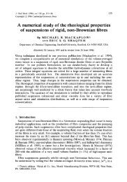
1.1 Transient shear viscosity <strong>of</strong> a <strong>polymer</strong> melt at low shear rates compared<br />
to a perfectly viscous liquid and an ideal elastic solid. . . . . . . . . . . 3<br />
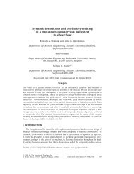
1.2 a) <strong>The</strong> storage and loss modulus for a single Maxwell mode with relaxation<br />
time τ. b) Linear rheology <strong>of</strong> a real <strong>polymer</strong> melt fitted with a<br />
spectrum <strong>of</strong> Maxwell modes [Venerus (2000)]. . . . . . . . . . . . . . . . 8<br />
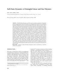
1.3 Non-linear shear and uniaxial extension <strong>of</strong> an LDPE melt 1810H showing<br />
extension hardening (solid shapes) and shear thinning (open shapes)<br />
[Suneel et al. (Submitted)]. . . . . . . . . . . . . . . . . . . . . . . . . . 10<br />
2.1 Sketch <strong>of</strong> an N-step freely jointed random walk . . . . . . . . . . . . . . 13<br />
2.2 In a Gaussian random walk monomers which are well separated along<br />
the chain may come into close contact. . . . . . . . . . . . . . . . . . . . 14<br />
2.3 <strong>The</strong> derivation <strong>of</strong> a molecular expression for stress . . . . . . . . . . . . 17<br />
2.4 Scaling <strong>of</strong> linear viscosity <strong>of</strong> a range <strong>of</strong> linear <strong>polymer</strong> melts against X w<br />
which is proportional to molecular weight. <strong>The</strong> scaling switches from a<br />
slope <strong>of</strong> 1 to the 3.4 “law” for <strong>entangled</strong> <strong>polymer</strong> melts. From Berry and<br />
Fox (1968). . . . . . . . . . . . . . . . . . . . . . . . . . . . . . . . . . . 21<br />
2.5 <strong>The</strong> many body problem <strong>of</strong> an <strong>entangled</strong> melt (a) reduced to a single<br />
chain problem by replacing the individual entanglements with a confining<br />
tube (b). . . . . . . . . . . . . . . . . . . . . . . . . . . . . . . . . . . . . 22<br />
2.6 A chain in an entanglement network (narrow line) and its corresponding<br />
primitive path (broad line). . . . . . . . . . . . . . . . . . . . . . . . . . 23<br />
2.7 Relaxation <strong>of</strong> oriented tube segments by reptation after a step strain . . 24<br />
2.8 a) Dynamic modulus as calculated by the pure reptation model. b) Experimental<br />
storage modulus for a range <strong>of</strong> narrow distribution polystyrenes.<br />
Z ranges between ≈ 44 and ≈ 0.6 entanglements [Onogi et al. (1970)]. . 26<br />
2.9 <strong>The</strong>oretical predictions <strong>of</strong> relaxation after a step strain. [Reproduced<br />
from Doi and Edwards (1986)] . . . . . . . . . . . . . . . . . . . . . . . 28<br />
iv
LIST OF FIGURES<br />
v<br />
2.10 Comparison <strong>of</strong> predicted and measured damping functions after a large<br />
step strain for different linear polystyrene solutions [Osaki et al. (1982)].<br />
<strong>The</strong> open and filled circles are data for different molecular weights and<br />
the tick directions indicate variations in concentration. . . . . . . . . . . 29<br />
2.11 Schematic representation <strong>of</strong> a constraint release event. . . . . . . . . . . 31<br />
2.12 Three relaxation mechanism available to an unbranched, <strong>entangled</strong> <strong>polymer</strong><br />
chain: reptation (a), constraint release (b) and retraction (c). . . . 33<br />
2.13 A three armed pom-pom molecule (q=3) . . . . . . . . . . . . . . . . . . 37<br />
2.14 Sketch <strong>of</strong> a random walk rescaled from N steps <strong>of</strong> length b to Z steps <strong>of</strong><br />
length a. . . . . . . . . . . . . . . . . . . . . . . . . . . . . . . . . . . . . 43<br />
2.15 Schematic showing a Brownian particle, subject to a spring force and<br />
moving in an array <strong>of</strong> vanishing and re-appearing obstacles. . . . . . . . 45<br />
3.1 Evolution <strong>of</strong> S xy for simple shear shear, ˙γ = 1sec −1 . Affine deformation<br />
corresponds to τ b = ∞ . <strong>The</strong> thin solid line corresponds to the value <strong>of</strong><br />
τ b for which the steady state value <strong>of</strong> S xy is maximised. . . . . . . . . . 51<br />
3.2 Evolution <strong>of</strong> S xy for nearly exponential shear with varying τ b values.<br />
α = 1sec −1 . . . . . . . . . . . . . . . . . . . . . . . . . . . . . . . . . . . 52<br />
3.3 Evolution <strong>of</strong> S xx − S yy for a planar extensional <strong>flow</strong>, ˙ɛ = 1sec −1 . . . . . 53<br />
3.4 Evolution <strong>of</strong> S xx − S yy for an exponential shear <strong>flow</strong>, α = 1sec −1 . . . . . 54<br />
3.5 Evolution <strong>of</strong> backbone stretch for a simple shear <strong>flow</strong>. τ b = 3sec, τ s =<br />
1sec and q = 5. . . . . . . . . . . . . . . . . . . . . . . . . . . . . . . . . 54<br />
3.6 Evolution <strong>of</strong> backbone stretch for an exponential shear <strong>flow</strong>, α = 1sec −1 ,<br />
τ b /τ s = 3. . . . . . . . . . . . . . . . . . . . . . . . . . . . . . . . . . . . 55<br />
3.7 Evolution <strong>of</strong> backbone stretch for a planar extensional <strong>flow</strong>. τ b = 3sec,<br />
τ s = 1sec and q=4. . . . . . . . . . . . . . . . . . . . . . . . . . . . . . . 56<br />
3.8 Evolution <strong>of</strong> shear stress in an exponential shear <strong>flow</strong>, α = 3sec −1 , τ b =<br />
3sec, τ s = 1sec and G 0 φ 2 b<br />
= 1. . . . . . . . . . . . . . . . . . . . . . . . . 58<br />
3.9 Pom-pom predictions compared to the experimental data for melt 1 <strong>of</strong><br />
Zülle et al. (1987). Filled shapes are nearly exponential shear data points<br />
and open shapes are true exponential shear data points. Solid lines are<br />
nearly exponential shear predictions and dashed lines are true exponential<br />
shear predictions for both (a) and (b). . . . . . . . . . . . . . . . . . 59<br />
3.10 Multimode pom-pom free parameter fit to planar extension data from<br />
Hachmann (1997). . . . . . . . . . . . . . . . . . . . . . . . . . . . . . . 61<br />
3.11 Comparison <strong>of</strong> multimode pom-pom predictions to experimental data for<br />
shear stress in true exponential shear from Venerus (2000). Solid curves<br />
are pom-pom predictions, shapes are data points and the dashed curve<br />
is the linear viscoelastic curve for simple shear. . . . . . . . . . . . . . . 62
vi<br />
LIST OF FIGURES<br />
3.12 Comparison <strong>of</strong> multimode pom-pom predictions to experimental data<br />
for first normal stress difference in true exponential shear from Venerus<br />
(2000). Solid curves are pom-pom predictions, shapes are data points<br />
and the dashed curve is the FLV curve for first normal stress difference<br />
in simple shear. . . . . . . . . . . . . . . . . . . . . . . . . . . . . . . . 63<br />
3.13 Free parameter fit <strong>of</strong> non-linear parameters <strong>of</strong> melt 1 using only nearly<br />
exponential shear data collected by Zülle (1987). . . . . . . . . . . . . . 66<br />
3.14 Comparison <strong>of</strong> pom-pom predictions using spec II with uniaxial extension<br />
data for melt 1 from Meissner (1972). . . . . . . . . . . . . . . . . . 67<br />
3.15 <strong>The</strong> 8 modes <strong>of</strong> melt 1 (see table 3.1) in nearly exponential shear for<br />
α = 0.01sec −1 . . . . . . . . . . . . . . . . . . . . . . . . . . . . . . . . . 68<br />
3.16 <strong>The</strong> 8 modes <strong>of</strong> melt 1 (see table 3.1) in uniaxial extension for ˙ɛ =<br />
0.01sec −1 . . . . . . . . . . . . . . . . . . . . . . . . . . . . . . . . . . . . 69<br />
3.17 Linear response <strong>of</strong> two batches <strong>of</strong> melt1810H: a)data collected by Venerus<br />
(2000) (melt 1810H) b) data collected by Suneel et al. (Submitted) (melt<br />
1810Hb). . . . . . . . . . . . . . . . . . . . . . . . . . . . . . . . . . . . . 70<br />
3.18 Experimental data and predictions for uniaxial extension <strong>of</strong> melt 1810Hb<br />
(filled shapes) and simple shear (open shapes) made using spec Ib which<br />
was obtained by fitting only to exponential shear data. . . . . . . . . . . 72<br />
3.19 Experimental data and predictions for true exponential and (filled shapes)<br />
and simple shear (open shapes) <strong>of</strong> melt 1810Hb made using spec IIb<br />
which was obtained by fitting only to uniaxial extension data. . . . . . . 73<br />
4.1 Two possibilities for the effect <strong>of</strong> a step deformation on the entanglement<br />
network. (a) <strong>The</strong> number <strong>of</strong> entanglements points is fixed and so the tube<br />
persistence length grows. (b) <strong>The</strong> tube persistence length remains fixed<br />
so Z grows in proportion with the primitive path length. . . . . . . . . . 76<br />
4.2 <strong>The</strong> effect <strong>of</strong> CCR on an unstretched segment (a) and a stretched segment<br />
(b). . . . . . . . . . . . . . . . . . . . . . . . . . . . . . . . . . . . . . . . 77<br />
4.3 Mechanism by which CCR relaxes chain stretch . . . . . . . . . . . . . . 78<br />
4.4 <strong>The</strong>ory predictions <strong>of</strong> steady state shear stress as a function <strong>of</strong> shear rate<br />
(c ν = 0.1). . . . . . . . . . . . . . . . . . . . . . . . . . . . . . . . . . . . 89<br />
4.5 Transient predictions for shear stress and normal stress against strain,<br />
γ, for start-up <strong>of</strong> simple shear. Model parameters: Z = 20, c ν = 0.1<br />
with shear rates from ˙γτ R = 21 to linear response. . . . . . . . . . . . . 90<br />
4.6 S(q) in steady shear for a range <strong>of</strong> shear rates. <strong>The</strong> two higher rate Rouse<br />
Weissenberg number are 0.42 and 6, respectively. Model parameters:<br />
Z = 20 and c ν = 0.1. Contours lines map the same value on each plot. . 91
LIST OF FIGURES<br />
vii<br />
4.7 Comparison with the Menezes and Graessley (1982) linear oscillatory<br />
shear data for three polybutadiene solutions: PBB, PBC and PBD, with<br />
c ν = 1.0 (a) and c ν = 0.1 (b). <strong>The</strong> model parameters, listed in the figure<br />
and in table 4.2, are the same for each molecular weight. . . . . . . . . . 93<br />
4.8 Comparison with Menezes and Graessley (1982) PBB shear viscosity (a)<br />
and first normal stress difference (b) data using parameters obtained<br />
only from linear rheology. . . . . . . . . . . . . . . . . . . . . . . . . . . 94<br />
4.9 Comparison with Menezes and Graessley (1982) PBB shear viscosity (a)<br />
and first normal stress difference (b) data using parameters obtained<br />
from linear rheology and R s = 2.0. . . . . . . . . . . . . . . . . . . . . . 96<br />
4.10 Comparison with Menezes and Graessley (1982) PBD shear viscosity (a)<br />
and first normal stress difference (b) data using parameters obtained<br />
from linear rheology and R s = 2.0. . . . . . . . . . . . . . . . . . . . . . 97<br />
4.11 Comparison with Hua et al. (1999) PS/TCP shear viscosity (a) and first<br />
normal stress difference (b) data using parameters obtained from linear<br />
rheology and R s = 2.0. . . . . . . . . . . . . . . . . . . . . . . . . . . . . 98<br />
4.12 Steady state shear stress and first normal stress difference <strong>of</strong> PS/TCP<br />
[Hua et al. (1999)] compared with model prediction for R s = 2.0. . . . . 99<br />
4.13 Derivation <strong>of</strong> CCR term for a stretched chain . . . . . . . . . . . . . . . 101<br />
5.1 A self dilute bimodal blend. <strong>The</strong> HMW chains are sufficiently rare that<br />
they do not self entangle. All constraint release events are produced by<br />
motion <strong>of</strong> the short chains. . . . . . . . . . . . . . . . . . . . . . . . . . 106<br />
5.2 Uniaxial extension <strong>of</strong> a set <strong>of</strong> bimodal blends [Hepperle (2001)] at 173.5 o C<br />
compared with model predictions (R s = 2.0). . . . . . . . . . . . . . . . 108<br />
5.3 A qualitative comparison <strong>of</strong> data (1) and theory (2) for bimodal blends <strong>of</strong><br />
<strong>entangled</strong> <strong>polymer</strong> solutions <strong>under</strong> strong shear including shear stress (a)<br />
and first normal stress difference (b). Experimental data by Osaki et al.<br />
(2000b) (on blend f80/850) with shear rates ranging from 1.165 − 0.0086<br />
sec −1 . <strong>The</strong>ory curves have shear rates in the range ˙γτ long<br />
R<br />
= 1 − 450. . 110
List <strong>of</strong> Tables<br />
1.1 <strong>The</strong> tensorial description <strong>of</strong> some simple <strong>flow</strong>s . . . . . . . . . . . . . . . 4<br />
2.1 Summary <strong>of</strong> the transformation from a discrete system to a continuous<br />
variable. . . . . . . . . . . . . . . . . . . . . . . . . . . . . . . . . . . . 16<br />
2.2 <strong>The</strong> pom-pom constitutive equation- differential approximation . . . . . 39<br />
3.1 Non-linear spectrum <strong>of</strong> melt 1 fitted to extensional rheology, from Inkson<br />
et al. (1999). . . . . . . . . . . . . . . . . . . . . . . . . . . . . . . . . . 58<br />
3.2 Non-linear spectrum <strong>of</strong> melt 1810H obtained by fitting to planar extension<br />
data from Hachmann (1997). . . . . . . . . . . . . . . . . . . . . . . 60<br />
3.3 Criterion <strong>of</strong> equation 3.22 applied to the linear spectrum <strong>of</strong> melt 1 and<br />
two non-linear spectra for melt 1. Spec I is a fit to uniaxial extension<br />
[Inkson et al. (1999)] and Spec II is a fit to the transient nearly exponential<br />
shear stress data collected by Zülle et al. (1987) . . . . . . . . . 65<br />
3.4 Criterion <strong>of</strong> equation 3.22 applied to the linear spectrum <strong>of</strong> melt 1810Hb<br />
and two non-linear spectra. Spec Ib is a fit to exponential shear data and<br />
Spec IIb is a fit to the transient uniaxial extensional data from Suneel<br />
et al. (Submitted). . . . . . . . . . . . . . . . . . . . . . . . . . . . . . . 71<br />
4.1 Closed system <strong>of</strong> equation including describing the dynamics <strong>of</strong> an ensemble<br />
<strong>of</strong> <strong>entangled</strong> linear <strong>polymer</strong>s including: contour length fluctuations,<br />
retraction, constraint release and variable number <strong>of</strong> entanglements. 85<br />
4.2 Material parameters for two polybutadiene solutions [Menezes and Graessley<br />
(1982)] and a polystyrene solution [Hua et al. (1999)]. Material parameters<br />
are as quoted in the original papers, fitted parameters are obtained<br />
from linear oscillatory shear and calculated parameters are computed<br />
from the other parameters. . . . . . . . . . . . . . . . . . . . . . . 93<br />
viii
Abstract<br />
<strong>The</strong> aim <strong>of</strong> this thesis is to investigate the use <strong>of</strong> microscopic molecular models <strong>of</strong><br />
<strong>entangled</strong> <strong>polymer</strong> <strong>fluids</strong> to predict the bulk properties <strong>of</strong> these materials. This is<br />
achieved by using and modifying refined versions <strong>of</strong> the tube model <strong>of</strong> Doi and Edwards<br />
to study both linear and branched <strong>polymer</strong>s.<br />
I investigate long chain branched <strong>polymer</strong>s using the “pom-pom” model <strong>of</strong> McLeish<br />
and Larson. In particular, I use this model as a tool to characterise industrial long chain<br />
branched materials using experimental data for exponential shear rheology. I highlight<br />
the successes <strong>of</strong> this approach and investigate the limitations <strong>of</strong> shear rheology relative<br />
to extensional measurements in this context.<br />
Expanding on recent work concerning the non-linear rheology <strong>of</strong> model, linear <strong>polymer</strong>ic<br />
<strong>fluids</strong> I develop a detailed microscopic model for the dynamics <strong>of</strong> these materials.<br />
<strong>The</strong> influence <strong>of</strong> chain stretch and contour length fluctuations are added to the Milner,<br />
McLeish and Likhtman implementation <strong>of</strong> convective constraint release. <strong>The</strong>se modifications<br />
allow an effective comparison with experimental data for model <strong>entangled</strong><br />
<strong>polymer</strong> solutions to be made. From this comparison I am able to draw conclusions<br />
concerning the ability <strong>of</strong> the tube model to predict non-linear rheology and to indicate<br />
<strong>flow</strong> regimes in which new physical insight appears to be necessary. I discuss possible<br />
future modifications to the model. Finally, I generalise the monodisperse model<br />
to cover non-linear <strong>flow</strong>s <strong>of</strong> self-dilute bimodal blends and compare predictions with<br />
experimental data in both shear and extension.<br />
ix
Acknowledgements<br />
I am very grateful to my supervisors, Tom McLeish and Oliver Harlen, for their<br />
help, support and guidance throughout my PhD. I have benefited greatly from their<br />
supervision. I also owe a large debt <strong>of</strong> gratitude to Alexei Likhtman with whom I have<br />
been collaborating for the last three years. I have learnt a considerable amount about,<br />
not only <strong>polymer</strong> dynamics, but research methodology from Alexei and the standard<br />
<strong>of</strong> my research has been considerably enhanced by Alexei’s influence.<br />
I would also like to thank Richard Blackwell for answering many <strong>of</strong> my questions<br />
about tube theory, particularly for branched <strong>polymer</strong>s and for helping me to <strong>under</strong>stand<br />
the tube model in the early part <strong>of</strong> my PhD. I am grateful to Peter Olmsted for general<br />
guidance during my PhD and for agreeing to act as my internal examiner. Thanks<br />
to Daniel Read for helping me attain greater appreciation <strong>of</strong> my work through his<br />
questioning and insightful suggestions.<br />
I also appreciate useful discussions with numerous researchers during my time at<br />
the KITP at the University <strong>of</strong> California, Santa Barbara. In particular I am grateful<br />
to Scott Milner and Ron Larson for guidance during this time. I would like to thank<br />
Pr<strong>of</strong>essor Marrucci and Giovanni Ianniruberto for taking the time to look over my work.<br />
I am also grateful to Pr<strong>of</strong>essor Marrucci for agreeing to act as external examiner.<br />
Thanks to Suneel for providing experimental rheology on melt1810Hb and collaborating<br />
with me during the analysis <strong>of</strong> these data. I am also grateful to David Venerus<br />
for kindly supplying his rheological data on both a model <strong>entangled</strong> linear solution and<br />
an industrial branched melt, both sets <strong>of</strong> data were particularly helpful in the development<br />
<strong>of</strong> this work. Thanks to Jens Hepperle for providing his blend data and for<br />
spending time discussing his work during his visit to Leeds and to Akanari Minegishi<br />
for kindly providing his blend data.<br />
I would also like to acknowledge all <strong>of</strong> the people involved in the µPP project. My<br />
involvement in this project has been useful in my development as a researcher. In<br />
particular, thanks to Timothy Nicholson for running this project. I also acknowledge<br />
Nat Inkson for help with the multimode pom-pom model.<br />
Thanks to Maureen Thompson and Beverly Robinson for help and support during<br />
my time at Leeds and to all other friends and colleagues at Leeds, particularly Anna<br />
x
ACKNOWLEDGEMENTS<br />
xi<br />
Maidens, Stuart Hill, Carole Whiting, Mike Ries, Alessio de Francesco and Simon<br />
Marlow.<br />
I also acknowledge financial support from the EPSRC and BP Chemicals and I<br />
would like to thank my contacts at BP, Choon Chai and Les Rose, for helping me to<br />
<strong>under</strong>stand the industrial relevance <strong>of</strong> my work and for providing a focus for my work.<br />
Finally, thanks to my family for help and support during my studies.
Chapter 1<br />
Introduction<br />
1.1 Overview<br />
Rheology is the study <strong>of</strong> the deformation <strong>of</strong> matter. In particular, it is the term<br />
used to describe the study <strong>of</strong> complex <strong>fluids</strong> such as <strong>polymer</strong> melts, <strong>polymer</strong> solutions<br />
and colloidal suspensions. <strong>The</strong> aim <strong>of</strong> theoretical rheology is to develop constitutive<br />
equations that relate stress within the material to its deformation history. Constitutive<br />
equations together with mass and momentum conservation can be used to predict<br />
the <strong>flow</strong> <strong>of</strong> the material. <strong>Molecular</strong> rheology aims to derive and <strong>under</strong>stand these<br />
constitutive equations from the <strong>under</strong>lying microscopic physics <strong>of</strong> the material.<br />
Polymer are large macromolecules. <strong>The</strong>y consist <strong>of</strong> many chemical repeat units<br />
covalently bonded into long chains. Chain with N = 10 2 − 10 4 repeat units can be<br />
synthesised and <strong>polymer</strong> <strong>of</strong> length N = 10 9 −10 10 occur in nature. <strong>The</strong> topology <strong>of</strong> the<br />
chain can vary from a simple linear chain to a complex branched structure. Chemically<br />
identical materials with the same molecular weight but different topologies <strong>of</strong>ten have<br />
radically different rheology. Conversely materials with different chemistries but with<br />
molecules <strong>of</strong> globally the same shape <strong>of</strong>ten exhibit evidence <strong>of</strong> universal behaviour.<br />
<strong>Molecular</strong> rheology <strong>of</strong> <strong>polymer</strong>s has a long history [Bird et al. (1977), Larson (1988),<br />
de Gennes (1979)]. However, work in this area has intensified in the last twenty years.<br />
Understanding <strong>polymer</strong> rheology is important not only from the point <strong>of</strong> view <strong>of</strong> fundamental<br />
science but because its applications <strong>of</strong>ten have very useful industrial consequences.<br />
A good <strong>under</strong>standing <strong>of</strong> the link between the molecular constituents <strong>of</strong> a<br />
<strong>polymer</strong> liquid and its rheological behaviour is a long term goal <strong>of</strong> molecular rheology.<br />
This would allow the production <strong>of</strong> materials with a rheology that is tailored to their<br />
application.<br />
<strong>The</strong>re are many processing problems which are thought to be avoidable if a material<br />
has the correct rheology. For example, in a film blowing process small areas <strong>of</strong> thinning<br />
in the film may grow in amplitude leading to rupture <strong>of</strong> the film. By changing the<br />
1
2 CHAPTER 1. INTRODUCTION<br />
extensional properties <strong>of</strong> the material this effect can be avoided. <strong>The</strong>oretical rheology<br />
is also increasingly being used to gain information about the molecular structure <strong>of</strong> a<br />
material from its rheological behaviour.<br />
<strong>The</strong> degree <strong>of</strong> branching in a <strong>polymer</strong> molecule is known to have strong influence on<br />
its rheology. For example highly branched <strong>polymer</strong> melts such as low density polyethylene<br />
(LDPE) exhibit strong strain hardening <strong>under</strong> extensional <strong>flow</strong>s. Strain hardening<br />
is defined as an increase in viscosity with strain and is a desirable processing property.<br />
However, melts comprising <strong>of</strong> mostly linear molecules rarely show strain hardening<br />
and are <strong>of</strong>ten strain s<strong>of</strong>tening. Thus the arrangement branch points or topology <strong>of</strong> a<br />
molecule can dominate its rheological behaviour.<br />
1.2 <strong>The</strong> stress tensor<br />
<strong>The</strong> goal <strong>of</strong> theoretical rheology is to relate the deformation history to macroscopic<br />
properties <strong>of</strong> the material. <strong>The</strong> mechanical stress exerted by the material in response<br />
to the deformation governs the <strong>flow</strong> <strong>of</strong> the material and so is one <strong>of</strong> the most frequently<br />
measured properties. Rheological constitutive equations make predictions <strong>of</strong> the stress<br />
tensor, σ. <strong>The</strong> Cartesian components, α, β, <strong>of</strong> the stress tensor are defined as the force<br />
≈<br />
per unit area in the α direction acting across a plane whose normal vector is in the β<br />
direction. In most material the stress tensor is symmetric. Asymmetry implies that<br />
microscopic points in the material experience a non-zero torque.<br />
1.3 Viscoelasticity<br />
Traditionally, the distinction between a liquid and a solid is clear. <strong>The</strong> response <strong>of</strong><br />
an ideal solid to deformation may be modelled by Hooke’s law. <strong>The</strong> stress response<br />
is proportional to the imposed strain and is independent <strong>of</strong> the strain rate. Thus the<br />
elastic energy supplied by the deformation is completely conserved. An ideal liquid<br />
has a Newtonian viscosity where the stress response is proportional to the imposed<br />
deformation rate and the total strain is irrelevant. In a Newtonian liquid the energy <strong>of</strong><br />
deformation is completely dissipated. Polymer liquids, amongst others, show behaviour<br />
which is part-way between these two extremes. This is demonstrated in figure 1.1 which<br />
compares the transient shear rheology <strong>of</strong> a <strong>polymer</strong> melt at low shear rates with the two<br />
ideal limits, showing elastic behaviour at early times, giving way to viscous behaviour<br />
at longer times. Note that at low rates different deformation rates superimpose onto a<br />
single, rate independent curve; this is not the case for more rapid deformations.
1.4. DEFORMATION KINEMATICS 3<br />
10 5<br />
Newtonian Viscosity<br />
10 4<br />
η 0<br />
(t)<br />
σ xy / γ . [Pa-sec]<br />
10 3<br />
Hooke’s Law<br />
10 2<br />
10 -2 10 -1 10 0 10 1<br />
time [sec]<br />
Figure 1.1: Transient shear viscosity <strong>of</strong> a <strong>polymer</strong> melt at low shear rates compared to<br />
a perfectly viscous liquid and an ideal elastic solid.<br />
1.4 Deformation kinematics<br />
Before attempting to derive a constitutive equation the deformation history imposed<br />
on the material must be defined. <strong>The</strong> response <strong>of</strong> a material depends on the geometry<br />
<strong>of</strong> the imposed deformation, therefore an adequate mathematical description <strong>of</strong> the<br />
deformation is essential. One way to achieve this is to specify the velocity field, v,<br />
imposed by the deformation on a material element at point r. However, only relative<br />
motion <strong>of</strong> material points are relevant, hence the velocity gradient tensor, κ<br />
≈<br />
, is usually<br />
a more relevant measure,<br />
κ (r, t) = (∇v(r,<br />
≈ t))T . (1.1)<br />
If κ<br />
≈<br />
does not depends on spatial position r then the <strong>flow</strong> is deemed a simple <strong>flow</strong>. A<br />
range <strong>of</strong> useful <strong>flow</strong>s such as shear and extension fall <strong>under</strong> this definition.<br />
Simple<br />
<strong>flow</strong>s are also more easily analysed theoretically and so data on these <strong>flow</strong>s is relatively<br />
abundant and reliable. In this thesis I will test constitutive models <strong>under</strong> simple<br />
<strong>flow</strong>s against experimental data as a prerequisite to <strong>under</strong>standing more complicated<br />
deformations.<br />
constitutive equations.<br />
<strong>The</strong> tensor κ<br />
≈<br />
is widely used to define the deformation in differential<br />
An alternative description <strong>of</strong> the deformation is the deformation gradient tensor,<br />
E<br />
≈<br />
, which relates the vector connecting two embedded points before the deformation,<br />
X, and after the deformation, X ′ ,<br />
X ′ = E.X. (1.2)<br />
≈<br />
<strong>The</strong> deformation gradient tensor is more commonly used in integral constitutive equations<br />
or to describe step deformations. Care must be exercised in the use <strong>of</strong> E since it<br />
contains information not only about the stretching caused by the deformation but also
4 CHAPTER 1. INTRODUCTION<br />
the rotation. Thus if the stress is a functional <strong>of</strong> E it is not guaranteed that a purely<br />
rotational deformation will not induce a stress in the material! A safer description is<br />
the finger tensor, C<br />
≈<br />
−1<br />
C<br />
≈ −1 = E<br />
≈ T .E<br />
≈<br />
. (1.3)<br />
This remains invariant <strong>under</strong> a solid body rotation. <strong>The</strong> velocity gradient tensor and<br />
the deformation gradient tensor are related by the following expression<br />
1.4.1 Volume conserving <strong>flow</strong>s<br />
∂<br />
∂t E ≈ (t′ , t) = κ<br />
≈<br />
.E<br />
≈<br />
. (1.4)<br />
In <strong>polymer</strong> <strong>fluids</strong> the bulk modulus, which controls the response to a change in volume,<br />
is typically many orders <strong>of</strong> magnitude large than the moduli for volume conserving<br />
deformations. Thus considerable deformation can be achieved with imposed stresses<br />
that are much smaller in magnitude than the bulk modulus. <strong>The</strong>se deformations can<br />
be taken to be volume conserving. In terms <strong>of</strong> the deformation gradient tensor the<br />
condition det E<br />
≈<br />
= 1 implies a volume conserving deformation. <strong>The</strong> same constraint on<br />
the velocity gradient tensor is Tr κ<br />
≈<br />
= 0.<br />
1.4.2 Some simple <strong>flow</strong>s<br />
Flow κ<br />
≈<br />
E<br />
≈<br />
Shear<br />
Uniaxial extension<br />
Planar extension<br />
⎛<br />
⎝<br />
⎛<br />
⎝<br />
0 ˙γ 0<br />
0 0 0<br />
0 0 0<br />
⎞<br />
⎠<br />
˙ɛ 0 0<br />
0 −˙ɛ/2 0<br />
0 0 −˙ɛ/2<br />
⎛<br />
⎝<br />
˙ɛ 0 0<br />
0 −˙ɛ 0<br />
0 0 0<br />
⎞<br />
⎠<br />
⎞<br />
⎠<br />
⎛<br />
⎝<br />
⎛<br />
⎝<br />
1 γ 0<br />
0 1 0<br />
0 0 1<br />
⎞<br />
⎠<br />
e ɛ ⎞<br />
0 0<br />
0 e −ɛ/2 0 ⎠<br />
0 0 e −ɛ/2<br />
⎛<br />
⎝<br />
e ɛ 0 0<br />
0 e −ɛ 0<br />
0 0 1<br />
⎞<br />
⎠<br />
Table 1.1: <strong>The</strong> tensorial description <strong>of</strong> some simple <strong>flow</strong>s<br />
A number <strong>of</strong> different simple <strong>flow</strong>s can be realised experimentally on <strong>polymer</strong> <strong>fluids</strong>,<br />
with varying degrees <strong>of</strong> difficulty. <strong>The</strong> most straightforward is a shear <strong>flow</strong> in which<br />
a uniform velocity gradient, ˙γ is imposed throughout the material. <strong>The</strong> shear strain,<br />
γ, is the total accumulated deformation (γ = ∫ ˙γ(t ′ )dt ′ ). <strong>The</strong> usual convention is for
1.4. DEFORMATION KINEMATICS 5<br />
<strong>flow</strong> to be in the x direction, the velocity gradient to act in the y direction, and the z<br />
direction to be parallel to the vorticity. Experimental data typically measure a range<br />
<strong>of</strong> relevant components <strong>of</strong> the stress tensor. <strong>The</strong> easiest component to measure is the<br />
force which directly opposes the shear, namely the shear stress, σ xy . Polymer <strong>fluids</strong><br />
also typically exert a force normal to the shear plane. This stress is measured relative<br />
to atmospheric pressure and is expressed as differences between diagonal components <strong>of</strong><br />
the stress tensor. Two independent stress differences can be defined: the first normal<br />
stress difference, N 1 = σ xx − σ yy and second normal stress difference, N 2 = σ yy −<br />
σ zz . Considerable experimental effort is required to produce reliable normal stress<br />
measurements in shear [Meissner (1972)]. Since shear contains both extensional and<br />
rotational characteristics, the principle stretching direction rotates as the <strong>flow</strong> proceeds.<br />
As a result, despite being a comparatively simple experiment, it can pose theoretical<br />
difficulties.<br />
Extensional <strong>flow</strong>s are rotation free. <strong>The</strong>y may be achieved by increasing the length<br />
<strong>of</strong> a sample exponentially in time, producing a linearly increasing velocity pr<strong>of</strong>ile. This<br />
constant velocity gradient is the extension rate, ˙ɛ, and from this the Hencky extensional<br />
strain, ɛ can be defined as ɛ = ∫ ˙ɛ(t ′ )dt ′ . <strong>The</strong> actual extensional strain is exp( ∫ ˙ɛdt).<br />
Conventionally, extension is taken to occur in the x direction. To maintain a fixed volume<br />
the two remaining directions can be allowed to contract equally, which is known<br />
as uniaxial extension. Alternatively, one direction can be held fixed, forcing the final<br />
direction to contract sufficiently to maintain the volume, which is called planar extension.<br />
For both <strong>flow</strong>s the first normal stress difference can be measured and in planar<br />
extension there is also a second normal stress difference. <strong>The</strong>se extensional <strong>flow</strong>s, particularly<br />
planar extension, are difficult experiments and the necessary equipment is only<br />
available in a limited number <strong>of</strong> laboratories. Other extensional <strong>flow</strong>s are feasible, such<br />
as bi-axial <strong>flow</strong>s, however data for such deformations are rare. <strong>The</strong> velocity gradient<br />
and deformation gradient tensors for these simple <strong>flow</strong>s are shown in table 1.1.<br />
1.4.3 Flow in complex geometries<br />
<strong>The</strong> aim <strong>of</strong> many constitutive equations is to produce reliable quantitative predictions<br />
for as many <strong>of</strong> the above simple <strong>flow</strong>s as possible, using the same parameters for each<br />
<strong>flow</strong>. This is, <strong>of</strong> course, conditional on the availability <strong>of</strong> suitable data for comparison.<br />
However, almost all <strong>flow</strong>s which are <strong>of</strong> industrial relevance are complex <strong>flow</strong>s. Many<br />
complex <strong>flow</strong>s will be a combination <strong>of</strong> shear and extensional deformations and so a<br />
model which captures these simple <strong>flow</strong>s might be expected to perform well for <strong>flow</strong>s<br />
<strong>under</strong> a complex geometry if a suitable numerical implementation can be found. However,<br />
this conjecture is by no means a guarantee. For example, many complex <strong>flow</strong>s
6 CHAPTER 1. INTRODUCTION<br />
have areas <strong>of</strong> reversing <strong>flow</strong>, which is not probed by the above <strong>flow</strong>s. For an example<br />
<strong>of</strong> such a computation using a finite element technique and a molecularly based<br />
constitutive equation which explicitly takes into account reversing <strong>flow</strong> see Lee et al.<br />
(2001).<br />
1.5 Linear rheology<br />
Linear rheology refers to experiments in which the applied strain is small (γ ≪ 1).<br />
<strong>The</strong>se measurements are useful for a variety <strong>of</strong> reasons. <strong>The</strong>y are relatively easy to<br />
realise experimentally and an isotropic material’s response is <strong>of</strong>ten insensitive to the<br />
geometry <strong>of</strong> the deformation. <strong>The</strong> experiments can also probe the material over a very<br />
wide range <strong>of</strong> timescales. When devising theories various linearised approximations are<br />
valid, which simplify the mathematics and allows more detailed theoretical ideas to be<br />
investigated.<br />
For sufficiently small strains the relationship between the stress and strain in a<br />
<strong>polymer</strong> liquid will be approximately linear. Also, the stress relaxation is characterised<br />
by a scalar function G(t) which is independent <strong>of</strong> the imposed strain. For a small step<br />
strain imposed at time t = 0 the stress at time t is given by<br />
σ<br />
≈<br />
(t) = C<br />
≈ −1 G(t). (1.5)<br />
Thus the stress contribution at time t due to a small strain at time t ′ is<br />
dσ(t) = d<br />
≈ dt ′ C −1 (t ′ )G(t − t ′ )dt ′ . (1.6)<br />
≈<br />
In the limit <strong>of</strong> small strains the time derivative <strong>of</strong> the the finger tensor can be written<br />
as<br />
d<br />
dt C −1 = κ + κ T . (1.7)<br />
≈ ≈ ≈<br />
Integrating equation 1.5 over the whole deformation history (t ′ = −∞...t) gives<br />
σ<br />
≈<br />
(t) =<br />
∫ t<br />
∞<br />
(<br />
)<br />
G(t − t ′ ) κ<br />
≈ (t′ ) + κ(t ′ ) T dt ′ . (1.8)<br />
≈<br />
Coleman and Noll (1961) demonstrated that if G(t) has “fading memory” then this is<br />
sufficient to produce the two extremes <strong>of</strong> elastic and viscous behaviour as outlined in<br />
section 1.3. Fading memory is defined by the conditions that G(t) is integrable and<br />
tends to zero sufficiently quickly as t → ∞ .
1.5. LINEAR RHEOLOGY 7<br />
1.5.1 Linear oscillatory shear<br />
Equation 1.5 can, in principle, be used to measure the relaxation modulus, G(t), directly.<br />
However, the step strain is never completely instantaneous so measured data at<br />
early times are unreliable and at long times the signal to noise ratio is weak, making the<br />
terminal behaviour difficult to obtain. A more effective approach is to use a continuous<br />
oscillating shear strain history. In complex notation this is expressed as<br />
γ(t) = R(γ max exp(iωt)). (1.9)<br />
Under this deformation history equation 1.5 gives<br />
σ xy (t) =<br />
∫ t<br />
−∞<br />
G(t − t ′ ) dγ<br />
dt ′ (t′ )dt ′ . (1.10)<br />
Substituting in the form <strong>of</strong> the oscillating shear history (equation 1.9) and changing<br />
the variable <strong>of</strong> integration gives<br />
(<br />
σ xy (t) = R iωγ(t)<br />
∫ ∞<br />
0<br />
)<br />
exp(−iωs)G(s)ds . (1.11)<br />
which can be rewritten as<br />
σ xy (t) = R (γ(t)G ∗ (ω)) . (1.12)<br />
where G ∗ (ω) is known as the complex modulus. Thus<br />
G ∗ (ω) = iω<br />
∫ ∞<br />
0<br />
e −iωt G(t)dt. (1.13)<br />
When the complex modulus is written as G ∗ = G ′ + iG ′′ it can be seen that G ∗ consists<br />
<strong>of</strong> a component which is in phase with the strain and one which is out <strong>of</strong> phase. <strong>The</strong><br />
in phase part, G ′ , is known as the storage or elastic modulus and the out <strong>of</strong> phase<br />
part, G ′′ , is the loss or dissipative modulus. A perfectly elastic solid <strong>of</strong> modulus G 0<br />
would have G ′ = G 0 and G ′′ = 0. In the case <strong>of</strong> a viscous liquid with viscosity η then<br />
G ′ = 0 and G ′′ = ωη since σ xy is in phase with the shear rate.<br />
For a viscoelastic<br />
material both G ′ and G ′′ are functions <strong>of</strong> the applied frequency, ω. In general, the<br />
loss modulus dominates at low frequencies, while the elastic modulus dominates at<br />
high frequencies. <strong>The</strong> material crosses over from viscous behaviour elastic behaviour at<br />
some intermediate frequency where G ′ = G ′′ . A simple form <strong>of</strong> the relaxation modulus,<br />
the Maxwell model, where G(t) = G 0 exp(−t/τ) which is characterised by a relaxation<br />
time, τ. <strong>The</strong> complex modulus for this model is given by,<br />
G ′ (ω) = G 0<br />
ω 2 τ 2<br />
1+ω 2 τ 2 , G ′′ (ω) = G 0<br />
ωτ<br />
1+ω 2 τ 2 . (1.14)
8 CHAPTER 1. INTRODUCTION<br />
In this case this cross-over frequency <strong>of</strong> G ′ and G ′′ is the exact reciprocal <strong>of</strong> the characteristic<br />
time.<br />
Although this simple model predicts the correct qualitative behaviour, to capture<br />
the quantitative behaviour <strong>of</strong> a real <strong>polymer</strong> fluid it is typically necessary to use a<br />
superposition <strong>of</strong> Maxwell modes.<br />
G(t) = ∑ i<br />
g i exp(−t/τ i ). (1.15)<br />
<strong>The</strong> set <strong>of</strong> moduli and corresponding times scales {g i , τ i } is known as the relaxation<br />
spectrum. A comparison <strong>of</strong> the linear rheology <strong>of</strong> a single exponential fluid to that <strong>of</strong><br />
a real <strong>polymer</strong> melt fitted with a relaxation spectrum is shown in figure 1.2. <strong>The</strong> melt<br />
is a polydisperse branched material known as melt 1810H [Venerus (2000)]. Note that<br />
the real melt has a considerably broader spectrum than the single Maxwell mode. In<br />
this more general case G ′ and G ′′ do not cross over at the reciprocal terminal time.<br />
Nevertheless, this cross over is <strong>of</strong>ten associated with a “characteristic relaxation time”<br />
<strong>of</strong> the material. It should be noted that the decomposition <strong>of</strong> G(t) into discrete Maxwell<br />
modes is not unique.<br />
10 1<br />
G’(ω)/G, G’’(ω)/G<br />
10 0<br />
10 -1<br />
10 -2<br />
G’<br />
G’’<br />
(a)<br />
10 -3<br />
10 -2 10 -1 10 0 10 1 10 2 10 3<br />
ωτ<br />
(b)<br />
Figure 1.2: a) <strong>The</strong> storage and loss modulus for a single Maxwell mode with relaxation<br />
time τ. b) Linear rheology <strong>of</strong> a real <strong>polymer</strong> melt fitted with a spectrum <strong>of</strong> Maxwell<br />
modes [Venerus (2000)].<br />
For a material with a wide range <strong>of</strong> relaxation times a correspondingly wide range<br />
<strong>of</strong> oscillation frequencies is needed to characterise the material fully. In practice, this<br />
is achieved, by appealing to the empirical principle <strong>of</strong> time-temperature superposition.<br />
This assumes that changing the experimental temperature is equivalent to shifting<br />
the frequency <strong>of</strong> the experiment.<br />
Thus an instrument’s limited range <strong>of</strong> frequency<br />
measurements can be extended by producing results at a range <strong>of</strong> temperatures and<br />
then shifting the data to produce a single temperature master curve. Materials which<br />
obey this principle are said to be thermo-rheologically simple.
1.6. NON-LINEAR RHEOLOGY 9<br />
1.5.2 Linear continuous shear<br />
Equation 1.10 can also be used to model a constant rate forward deformation provided<br />
that the deformation rate is small in comparison to the longest relaxation time <strong>of</strong> the<br />
material. For a continuous shear deformation commencing at time t = 0 the model<br />
predicts,<br />
σ xy (t) =<br />
∫ t<br />
0<br />
G(t − t ′ ) ˙γdt ′ . (1.16)<br />
In these shear experiments the transient shear viscosity, η + (t) = σ xy (t)/ ˙γ, is <strong>of</strong>ten<br />
plotted as a function <strong>of</strong> time. In this plot a Newtonian fluid would show a constant<br />
response at all deformation rates (see figure 1.1). For a linear viscoelastic fluid, whose<br />
constitutive equation is given by equation 1.8, the transient shear viscosity, η 0 (t), will<br />
be independent <strong>of</strong> the applied shear rate. This behaviour is seen in <strong>polymer</strong>ic <strong>fluids</strong><br />
at low shear rates (less than the reciprocal <strong>of</strong> the longest relaxation time) and also at<br />
early times when the applied strain, ˙γt, is small. Under these conditions the material<br />
is described as being in linear response. <strong>The</strong> master curve can be obtained from the<br />
linear relaxation spectrum. If G(t) is taken to be the sum <strong>of</strong> independent Maxwell<br />
modes (equation 1.15) then equation 1.16 gives<br />
η 0 (t) = ∑ i<br />
g i τ i [1 − exp(−t/τ i )] . (1.17)<br />
At higher deformation rates the transient curves <strong>of</strong> <strong>polymer</strong>ic <strong>fluids</strong> <strong>of</strong>ten deviate from<br />
linear response at strains <strong>of</strong> order one. <strong>The</strong> form <strong>of</strong> the deviation can be used to classify<br />
the material’s non-linear response.<br />
A similar transient viscosity, based on the first normal stress difference, can be<br />
defined for extensional <strong>flow</strong>s η + E (t) = N 1/˙ɛ. Using equation 1.8 it can be shown that,<br />
for a linear viscoelastic fluid in uniaxial extension, η + E (t) = 3η 0(t).<br />
1.6 Non-linear rheology<br />
Non-linear rheology refers to <strong>flow</strong>s in which the strain rates and accumulated strains<br />
are large. More specifically, the strain rate must be faster than some characteristic<br />
time <strong>of</strong> the material, usually the terminal time. Strains must be <strong>of</strong> order one or larger<br />
to observe non-linear effects. <strong>The</strong>se <strong>flow</strong>s are useful for a number <strong>of</strong> reasons. Nonlinear<br />
measurements on <strong>polymer</strong> liquids <strong>of</strong>ten show very striking behaviour and can,<br />
consequently, be more sensitive to molecular details than weaker deformations. For<br />
example, the extensional rheology <strong>of</strong> a polydisperse system can be strongly dependent<br />
on the high molecular weight tail <strong>of</strong> the distribution. A material’s response to different<br />
deformation geometries is <strong>of</strong>ten qualitatively different <strong>under</strong> non-linear deformations.
10 CHAPTER 1. INTRODUCTION<br />
This provides a good testing ground for any non-linear theory. For example <strong>polymer</strong><br />
liquids are <strong>of</strong>ten strain hardening in extension and thinning in shear. In figure 1.3 at<br />
10 6<br />
η Shear<br />
, η Extension<br />
(Pa-s)<br />
10 5<br />
10 4<br />
10 3<br />
3η 0<br />
(t)<br />
0.003<br />
0.01<br />
0.03<br />
0.1<br />
0.3<br />
1.0<br />
3.0<br />
10.0<br />
10 -1 10 0 10 1 10 2 10 3 10 4<br />
t (s)<br />
η 0 (t)<br />
Figure 1.3: Non-linear shear and uniaxial extension <strong>of</strong> an LDPE melt 1810H showing<br />
extension hardening (solid shapes) and shear thinning (open shapes) [Suneel et al.<br />
(Submitted)].<br />
small strains the extension viscosity is three times the shear viscosity. However, at high<br />
rates the extension data rise above the low rate extension curve whereas the high rate<br />
shear data fall below the corresponding limiting curve. Many industrially relevant <strong>flow</strong>s<br />
involve very large strains and strain rates. To model these <strong>flow</strong>s non-linear rheology<br />
must be <strong>under</strong>stood.<br />
1.6.1 A simple empirical non-linear model<br />
A simple non-linear equation can be derived from the approach used in section 1.5 by<br />
avoiding the linear approximation <strong>of</strong> the time derivative <strong>of</strong> finger tensor. Equation 1.6<br />
can be integrated by parts to give<br />
∫<br />
d<br />
t<br />
dt σ dG(t − t ′ )<br />
= −<br />
≈<br />
∞ dt ′ C −1 (t ′ )dt ′ . (1.18)<br />
≈<br />
which is known as the Lodge equation. Furthermore this equation can be differentiated<br />
with respect to t to obtain a differential equation. For simplicity I also take the form<br />
<strong>of</strong> the relaxation modulus to be G(t) = G exp(−t/τ)<br />
d<br />
dt σ − κ.σ − σ.κ T = − 1 ) (σ − GI . (1.19)<br />
≈ ≈ ≈ ≈ ≈ τ ≈ ≈
1.7. ALTERNATIVE EXPERIMENTAL TECHNIQUES 11<br />
This can be written more compactly as<br />
∇<br />
σ = − 1 ) (σ − GI . (1.20)<br />
≈ τ ≈ ≈<br />
Where the operator ∇ is known as an upper convected Maxwell derivative and the<br />
general form <strong>of</strong> constitutive equation is called an upper convected Maxwell equation. In<br />
the non-linear regime the choice <strong>of</strong> equation 1.5 as the starting point <strong>of</strong> the derivation is<br />
arbitrary and other combinations <strong>of</strong> the finger tensor are equally permissible. Under this<br />
empirical approach these choices can only be vindicated by comparison with observed<br />
phenomena.<br />
If the relaxation modulus is taken to be a sum over exponential Maxwell modes<br />
(equation 1.15) then equation 1.20 can be solved for an independent set <strong>of</strong> non-linear<br />
Maxwell modes to produce stress predictions.<br />
1.7 Alternative experimental techniques<br />
Although the measurement <strong>of</strong> mechanical stresses is the most common and arguably<br />
the most industrially relevant measurement there are a range <strong>of</strong> additional experimental<br />
techniques which can be used to provide information about <strong>polymer</strong> <strong>fluids</strong> <strong>under</strong> <strong>flow</strong>.<br />
From an empirical point <strong>of</strong> view these measurements provide additional phenomena<br />
that must be explained. However, they are particularly useful in the field <strong>of</strong> molecular<br />
rheology since many <strong>of</strong> the experiments <strong>of</strong>fer a more direct probe <strong>of</strong> the molecular<br />
dynamics. Examples <strong>of</strong> these experiment include small angle neutron scattering (SANS)<br />
[Müller et al. (1993), McLeish et al. (1999)], NMR [Cormier and Callaghan (2002)],<br />
neutron spin echo [Wischnewski et al. (2002)] and dielectric relaxation [Watanabe et al.<br />
(2002)]. <strong>The</strong> use <strong>of</strong> these measurements in the verification and development <strong>of</strong> molecular<br />
models is a relatively new approach but they appear to provide new insight into the<br />
behaviour <strong>of</strong> <strong>polymer</strong>s <strong>under</strong> <strong>flow</strong> [McLeish (2002)].
Chapter 2<br />
Introduction to molecular<br />
rheology<br />
2.1 Overview<br />
In this chapter I will introduce some ideas used in the prediction <strong>of</strong> rheological properties<br />
from microscopic theories <strong>of</strong> the motion <strong>of</strong> <strong>polymer</strong> molecules. This section presents<br />
established knowledge, much <strong>of</strong> which is contained in the books <strong>of</strong> de Gennes (1979),<br />
Doi and Edwards (1986), Larson (1988) and Cates and Evans (2000).<br />
2.2 Gaussian chains<br />
Many <strong>of</strong> the more advanced models for <strong>polymer</strong> dynamics make use <strong>of</strong> the statistics <strong>of</strong><br />
Gaussian chains. Gaussian chains have a useful mathematical simplicity and, despite<br />
the seemingly crude assumptions necessary for their use, they form a valid model <strong>under</strong><br />
many circumstances.<br />
2.2.1 Random walk model<br />
<strong>The</strong> random walk model views a <strong>polymer</strong> chain as a series <strong>of</strong> N connected, straight<br />
bonds <strong>of</strong> fixed length, b. Each <strong>of</strong> these bonds points in a random direction chosen from<br />
an isotropic distribution. Thus each step is totally uncorrelated with the previous step.<br />
This type <strong>of</strong> model is known as a freely jointed random walk and is shown in figure 2.1.<br />
Using the fact that each step is independent <strong>of</strong> the previous step it is straightforward<br />
to show that the end to end vector r has the following average properties.<br />
〈r〉 = 0<br />
〈<br />
r<br />
2 〉 = Nb 2 .<br />
(2.1)<br />
12
¡ ¡ ¡ ¡ ¡ ¡ ¡<br />
¡ ¡ ¡ ¡ ¡ ¡ ¡<br />
2.2. GAUSSIAN CHAINS 13<br />
¡ ¡ ¡ ¡ ¡ ¡ ¡<br />
b<br />
Figure 2.1: Sketch <strong>of</strong> an N-step freely jointed random walk<br />
R<br />
In addition, r is the sum <strong>of</strong> many random vectors <strong>of</strong> fixed length so, if N is sufficiently<br />
large, the probability density <strong>of</strong> r can be shown to tend to the following Gaussian<br />
distribution.<br />
Ψ(r) =<br />
2.2.2 Justification <strong>of</strong> the model<br />
( ) 3 3/2 )<br />
2πNb 2 exp<br />
(− 3r2<br />
2Nb 2 . (2.2)<br />
Some limitations <strong>of</strong> using Gaussian statistics to model the static properties <strong>of</strong> a <strong>polymer</strong><br />
chain are immediately apparent. A random walk <strong>of</strong> N steps <strong>of</strong> length b has a maximum<br />
possible end to end vector length <strong>of</strong> Nb corresponding to the case in which all <strong>of</strong> the<br />
bonds point in the same directions. Yet equation 2.2 assigns a non-zero probability to<br />
vector lengths in excess <strong>of</strong> this value. In practice, as long as N is reasonably large the<br />
probability <strong>of</strong> achieving these unphysically large end to end vectors is small enough to<br />
have a negligible effect on the chain properties. Under very large and rapid deformations<br />
a chain can be unravelled sufficiently to approach its maximum extensibility and in this<br />
case a more detailed counting <strong>of</strong> microstates must be used.<br />
Why take each monomer step to be freely jointed? <strong>The</strong>re are examples <strong>of</strong> more<br />
detailed models <strong>of</strong> long chain molecules in which each bond direction is constrained to<br />
be related to the previous bond in the chain. However, so long as these correlation<br />
decay over some distance along the chain and the chain length is long compared with<br />
this distance, the value <strong>of</strong> 〈 r 2〉 still scales with the first power <strong>of</strong> N. <strong>The</strong> effect <strong>of</strong> these<br />
local bond correlations merely renormalises the bond length, b. This renormalised step<br />
length is known as the Kuhn statistical step length. <strong>The</strong> results presented so far still<br />
hold for weakly correlated random walks provided b is Kuhn step length rather than<br />
the raw bond length value.<br />
Another key assumption for the use <strong>of</strong> Gaussian chains is that interactions between<br />
two points which are well separated along the chain are neglected. Although plausible
14 CHAPTER 2. INTRODUCTION TO MOLECULAR RHEOLOGY<br />
Figure 2.2: In a Gaussian random walk monomers which are well separated along the<br />
chain may come into close contact.<br />
arguments for neglecting bond correlations along the chain can be made this is insufficient<br />
to allow the total neglect <strong>of</strong> all inter-monomer interactions. As a chain loops<br />
over on itself is possible for two monomers from separate parts <strong>of</strong> the chain to come<br />
into close contact. Figure 2.2 shows such a configuration. In fact Gaussian chains have<br />
no mechanism to prevent monomers from passing through each other. If the chain<br />
is, more realistically, to be considered to consist <strong>of</strong> monomers with a finite width as<br />
well as length, then configurations such as that in figure 2.2 should be discounted as<br />
allowable microstates <strong>of</strong> the <strong>polymer</strong> chain. This considerably changes the static properties<br />
<strong>of</strong> the chain. For example if a chain has a small value <strong>of</strong> r 2 then it is likely to<br />
contain many loops in which separate monomers are close to each other. Many <strong>of</strong> the<br />
microstates corresponding to this value <strong>of</strong> r 2 , which were allowed for phantom chains,<br />
must be neglected if the chain is self-avoiding. In contrast extended configurations<br />
lose fewer microstates this way since they contain fewer loops. Thus the chain end to<br />
end distribution function becomes more biased towards extended distributions and the<br />
chain becomes swollen. This is, indeed, the case for single chains, however, in melts<br />
and concentrated solutions the chain must also avoid interactions with neighbouring<br />
chains as well as with itself. If the monomer density is constant throughout the melt<br />
then configurations are lost equally for all end to end vectors and so Gaussian statistics<br />
are maintained. This unexpected result was first <strong>under</strong>stood by Flory (1953) and has<br />
been verified experimentally by scattering experiments on linear <strong>polymer</strong> melts (see for<br />
example Cotton et al. (1974)).<br />
2.2.3 Bead spring model<br />
Equation 2.2 can be used to derive a force extension law for a Gaussian chain. For a<br />
given end to end vector, r, the number <strong>of</strong> chain arrangements that achieve this vector,<br />
Ω, is given by<br />
Ω(r) = Ω total Ψ(r). (2.3)
2.2. GAUSSIAN CHAINS 15<br />
This leads to an expression for the chain entropy, S = k B ln Ω, as a function <strong>of</strong> end to<br />
end vector.<br />
S = S 0 − 3k Br 2<br />
2Nb 2 . (2.4)<br />
Since each Kuhn segment is freely jointed there is no internal energy cost associated<br />
with any distribution <strong>of</strong> the chain. As a consequence, the chain’s free energy, F, is<br />
purely entropic.<br />
F(r) = 3k BT r 2<br />
2Nb 2 − F 0 . (2.5)<br />
This free energy is converted to a force by applying the grad operator,<br />
F(r) = − 3k BT<br />
r. (2.6)<br />
Nb2 If the chain is divided into N + 1 beads each connected by a spring then the forceextension<br />
law for each spring is<br />
F(r n ) = − 3k BT<br />
b 2 r n . (2.7)<br />
where r is the vector connecting beads n and n − 1. Thus the global properties <strong>of</strong> a<br />
Gaussian random walk are the same as a series <strong>of</strong> N + 1 beads connected by springs<br />
with spring constants given by equation 2.7.<br />
2.2.4 Rouse dynamics<br />
With the bead spring model established as valid for the static properties <strong>of</strong> <strong>polymer</strong><br />
chains it becomes natural to use the same ideas to model <strong>polymer</strong> dynamics. This model<br />
was originally proposed by Rouse (1953) and still <strong>under</strong>pins many modern theories. <strong>The</strong><br />
<strong>polymer</strong> chain is modelled as a collection <strong>of</strong> N + 1 beads connected by springs with<br />
a spring constant <strong>of</strong> 3k B T/b 2 . <strong>The</strong> drag on a bead due to the surrounding solvent is<br />
proportional to the relative velocity <strong>of</strong> the bead and its surrounding solvent, with the<br />
friction constant ζ 0 per monomer. Interactions between the beads mediated by solvent,<br />
namely hydrodynamics interactions, are neglected. Topological interactions between<br />
the chains on different parts <strong>of</strong> the same chain are also neglected. Thus the beads are<br />
not prohibited from passing through each other. This seemingly unphysical model is<br />
still valid and useful <strong>under</strong> certain conditions (see section 2.2.8 for a discussion <strong>of</strong> this).<br />
<strong>The</strong> bead positions are labelled R 0 ....R N and the force due to the nth spring is<br />
calculated using r n = R n − R n−1 . Each bead experiences forces due to: the adjoining<br />
springs, drag from its surroundings and random Brownian collisions. Thus the force
16 CHAPTER 2. INTRODUCTION TO MOLECULAR RHEOLOGY<br />
balance on bead n is given by<br />
ζ 0<br />
( ∂Rn<br />
∂t<br />
− κ<br />
≈<br />
.R n<br />
)<br />
= − 3k BT<br />
b 2 (2R n − R n+1 − R n−1 ) + f n (t). (2.8)<br />
Here the viscous forces are assumed to dominate over inertial forces so the m ∂2 R<br />
term<br />
∂t 2<br />
is dropped. <strong>The</strong> random force experienced by each bead due to collisions with the<br />
surrounding is represented by the force f n . <strong>The</strong> beads at the chain ends are connected<br />
to just one other bead and so experience a spring force from just one neighbour. To<br />
ensure that equation 2.8 holds for the end bead, hypothetical beads at n = 0, N + 1<br />
are included with zero extension. This leads to the following boundary conditions.<br />
R 0 = R 1 R N = R N+1 . (2.9)<br />
In principle equations 2.8 and 2.9 define a system that may be solved to give the<br />
trajectories <strong>of</strong> each beads within the Rouse chain. However, in practice it is <strong>of</strong>ten more<br />
convenient to take the continuous limit <strong>of</strong> this system (see section 2.2.5). In either case a<br />
further derivation is required to convert information about the chain configuration into<br />
a quantity which can be measured experimentally. I will demonstrate such a calculation<br />
in section 2.2.6<br />
2.2.5 Continuous limit<br />
It is <strong>of</strong>ten more convenient to describe a chain contour in terms <strong>of</strong> a continuous variable<br />
rather than a set <strong>of</strong> discrete points. When describing a rouse chain by a set <strong>of</strong> N beads<br />
it is required that the system be independent <strong>of</strong> the number <strong>of</strong> beads used in the<br />
solution. One way <strong>of</strong> achieving this is to take the limit <strong>of</strong> the number <strong>of</strong> beads tending<br />
to infinity. This leads to a description <strong>of</strong> the chain contour in terms <strong>of</strong> a continuous<br />
variable rather than a set <strong>of</strong> discrete points. Thus R n becomes R(n), terms involving<br />
next neighbour differences become derivative with respect to the continuous variable<br />
n and sums can be replaced by integrals (see table 2.1) <strong>The</strong> derivatives are obtained<br />
Discrete<br />
Continuous<br />
R n → R(n)<br />
∂R<br />
R n − R n−1 →<br />
∂n<br />
R n+1 + R n−1 − 2R n →<br />
∂ 2 R<br />
∂n 2<br />
δ nm → δ(n − m)<br />
∑ m ′<br />
n=m<br />
Table 2.1: Summary <strong>of</strong> the transformation from a discrete system to a continuous<br />
variable.<br />
→<br />
∫ m ′<br />
m<br />
dn
2.2. GAUSSIAN CHAINS 17<br />
L<br />
α<br />
β<br />
Figure 2.3: <strong>The</strong> derivation <strong>of</strong> a molecular expression for stress<br />
through finite difference definitions <strong>of</strong> the derivative which become exact in the limit<br />
<strong>of</strong> large N.<br />
2.2.6 <strong>Molecular</strong> expression for stress<br />
Equations 2.8 and 2.9 define a system that can be solved to find the molecular shape,<br />
R(s). From this information a variety <strong>of</strong> measurable quantities can be deduced, including<br />
the macroscopic stress tensor, σ. To compute σ for an ensemble <strong>of</strong> Gaussian<br />
≈ ≈<br />
chains the configuration <strong>of</strong> the chains must be known above some length-scale and<br />
chain segments on length-scales below this scale must be locally at equilibrium. In this<br />
calculation the cut <strong>of</strong>f length-scale is taken to be the Kuhn step length, b, although<br />
<strong>of</strong>ten in practice, the molecule is only disturbed from equilibrium on length-scales much<br />
larger than this. This choice <strong>of</strong> length-scale corresponds to dividing the molecule into<br />
N subchains.<br />
An expression for the stress is obtained by considering a cube <strong>of</strong> length L, where<br />
L is large enough to be much greater than the end to end vector <strong>of</strong> a subchain and is
18 CHAPTER 2. INTRODUCTION TO MOLECULAR RHEOLOGY<br />
small enough that all quantities can be considered to be homogeneous inside the cube.<br />
This situation is illustrated in figure 2.3. A subchain inside such a cube has its end to<br />
end vector denoted by r n where n labels the bead number. This subchain will cross a<br />
plane with normal in the α direction with probability r nα /L (α and β denote Cartesian<br />
components). If the chain carries a tension F n then the force in the β direction caused<br />
by this chain is F nβ . Note that both the end to end vector and the tension depend<br />
upon bead number. <strong>The</strong> total <strong>polymer</strong> contribution to stress is obtained by summing<br />
over all subchains inside the cube. This is achieved by summing over all chains and all<br />
bead numbers,<br />
σ αβ = 1 L 3<br />
∑<br />
chains,n<br />
r nα F nβ . (2.10)<br />
If the cube contains enough chains the sum over chains can be replaced by an ensemble<br />
average 〈...〉. This average is over all subchains with the same bead position within the<br />
same course-graining volume. An average over bead positions is not taken. <strong>The</strong> cube<br />
will contain cL 3 /N chains (c is the monomer density) thus the <strong>polymer</strong> contribution<br />
to stress inside this cube is<br />
σ αβ = c ∑<br />
〈r nα F nβ 〉 . (2.11)<br />
N<br />
n<br />
<strong>The</strong> tension, F n , is a known function <strong>of</strong> the local chain configuration (equation 2.7).<br />
Taking the continuous limit allows the sum over beads to be replaced by an integral<br />
along the chain contour and r n by the first derivative <strong>of</strong> the chain space-curve. This<br />
leads to the final expression for the stress<br />
σ αβ = c N<br />
3k B T<br />
b 2<br />
∫ N<br />
0<br />
〈 ∂Rα<br />
∂n<br />
〉<br />
∂R β<br />
dn. (2.12)<br />
∂n<br />
2.2.7 Non-linear constitutive equation<br />
A non-linear constitutive equation can be constructed from the Rouse model in the<br />
following way [Larson (1988)]. Beginning with the continuous representation <strong>of</strong> equation<br />
2.8<br />
( )<br />
∂R<br />
ζ 0<br />
∂t − κ .R = 3k BT<br />
≈ b 2<br />
∂ 2 R<br />
+ f(n, t). (2.13)<br />
∂n2 <strong>The</strong> quantity f(n, t) represents the local Brownian forces acting on an individual beads,<br />
which are assumed to be random and isotropically distributed. Thus the forces act<br />
equally in all directions and are uncorrelated in time and position along the chain.<br />
<strong>The</strong> size <strong>of</strong> the force is fixed by insisting that all points on the chain are in thermal
2.2. GAUSSIAN CHAINS 19<br />
equilibrium with the surroundings. This gives<br />
〈f(n, t)〉 = 0<br />
〈<br />
f(n, t)f(n ′ , t) 〉 = 2ζ 0 k B T δ(n − n ′ )I<br />
≈<br />
.<br />
(2.14)<br />
In the continuous limit the boundary conditions <strong>of</strong> equation 2.9 become<br />
∂R<br />
∂n<br />
⏐ = 0. (2.15)<br />
n=0,N<br />
It is convenient to take a Fourier series <strong>of</strong> equation 2.13 in order to obtain a system <strong>of</strong><br />
ODEs. <strong>The</strong> equation is diagonalized by the following transformation.<br />
X p (t) = 1 N<br />
∫ N<br />
0<br />
R(n, t) cos<br />
( pπn<br />
)<br />
dn. (2.16)<br />
N<br />
which has the inverse transform<br />
R(n, t) = X 0 + 2<br />
∞∑ ( pπn<br />
)<br />
X p cos . (2.17)<br />
N<br />
p=1<br />
Thus the spacecurve describing the chain contour is decomposed into a Fourier series<br />
with vector amplitudes, X p . Applying this transformation to equation 2.13 gives<br />
∂X p<br />
∂t<br />
= κ<br />
≈<br />
.X p − p2<br />
τ R<br />
X p + g p (t). (2.18)<br />
where g p (t) is the p th Fourier component <strong>of</strong> the random force f(n, t) and the Rouse<br />
time, τ R , is given by<br />
τ R = ζ 0b 2 N 2<br />
3π 2 k B T . (2.19)<br />
<strong>The</strong> second moment <strong>of</strong> the action <strong>of</strong> Brownian forces on the Rouse modes is obtained<br />
by<br />
〈<br />
gp (t)g q (t ′ ) 〉 = 1<br />
ζ 2 0 N 2 ∫ N<br />
0<br />
∫ N<br />
= k BT<br />
ζ 0 N δ(t − t′ )δ pq I<br />
≈<br />
.<br />
0<br />
〈<br />
f(n, t)f(n ′ , t ′ ) 〉 ( pπn<br />
)<br />
cos cos<br />
N<br />
In terms <strong>of</strong> the Rouse modes, the stress (equation 2.12) becomes<br />
( qπn<br />
′<br />
N<br />
)<br />
dndn ′<br />
(2.20)<br />
σ = 3k BT c 2π 2 ∑<br />
p 2<br />
≈ Nb 2 〈X p X p 〉 . (2.21)<br />
N
20 CHAPTER 2. INTRODUCTION TO MOLECULAR RHEOLOGY<br />
Thus to compute the stress an expression for the second moment <strong>of</strong> the Rouse mode<br />
amplitude is required.<br />
Note that cross correlations between the modes (p ≠ q) do<br />
not contribute to the stress. In fact an independent set <strong>of</strong> ODEs for 〈X p X p 〉 can be<br />
found and so the cross correlations can be ignored. <strong>The</strong> set <strong>of</strong> differential equations is<br />
obtained from equation 2.18 by using an Ito-Stratonovich relation (see appendix 2.I for<br />
a discussion <strong>of</strong> this result)<br />
〈g p (t)X p (t)〉 = k BT<br />
2ζ 0 N I ≈ . (2.22)<br />
Taking the second moment <strong>of</strong> equation 2.18 and substituting equation 2.22 gives<br />
∂ 〈X p X p 〉<br />
∂t<br />
= κ<br />
≈<br />
. 〈X p X p 〉 + 〈X p X p 〉 .κ<br />
≈ T − 2p2<br />
τ R<br />
〈X p X p 〉 + k BT<br />
Nζ 0<br />
I<br />
≈<br />
. (2.23)<br />
By writing σ<br />
≈ p<br />
= 2π2<br />
Nb 2 p 2 〈X p X p 〉 the stress can expressed as a sum <strong>of</strong> mode contributions<br />
σ<br />
≈<br />
= 3k BT c<br />
N<br />
∑<br />
σ (2.24)<br />
≈ p.<br />
where each <strong>of</strong> these components obeys an independent upper convected Maxwell (UCM)<br />
equation (see section 1.6.1 for an empirical argument which leads to a UCM model for<br />
<strong>polymer</strong> <strong>fluids</strong>)<br />
with relaxation time τ p = 1/2p −2 τ R .<br />
p<br />
∇<br />
σ = −<br />
(σ 2p2 − 1 )<br />
≈ p τ R ≈ p 3 I . (2.25)<br />
≈<br />
Thus each stress component makes an equal<br />
contribution to the stress but higher modes have much faster relaxation times (τ p ∼<br />
p −2 ). This result justifies the assumption that small length-scales <strong>of</strong> the molecules are<br />
locally at equilibrium as used in the derivation <strong>of</strong> an expression for stress.<br />
It is worth noting that the above result can be derived without using the Ito-<br />
Stratonovich relation (equation 2.22). This is achieved by direct integration <strong>of</strong> equation<br />
2.18 over time and then taking the square <strong>of</strong> the resulting expression before averaging.<br />
However, the Ito-Stratonovich relation is useful in that it allows the derivation <strong>of</strong><br />
differential, as opposed to integral, constitutive equations.<br />
2.2.8 Validity <strong>of</strong> the Rouse model<br />
As discussed above, some, apparently drastic, simplifications are made in deriving the<br />
Rouse model. However, <strong>under</strong> some circumstances these approximations appear to be<br />
valid. Although the neglect <strong>of</strong> hydrodynamic interactions causes the model to fail for<br />
dilute solutions, experimental evidence suggests that these interactions are screened in<br />
concentrated <strong>polymer</strong> <strong>fluids</strong> [Ferry (1980)]. Yet applying the model to the dynamics<br />
<strong>of</strong> concentrated <strong>fluids</strong> seems to bring the phantom chain assumption into question.
2.3. DOI-EDWARDS MODEL OF ENTANGLED POLYMERS 21<br />
This problem can be averted by considering certain specific regimes <strong>of</strong> melt dynamics.<br />
Where <strong>polymer</strong> chains are shorter than some critical mass or time-scales are shorter<br />
than some critical time then the Rouse model appears to describe these systems well.<br />
However in more general situations one must explicitly take into account the topological<br />
interactions <strong>of</strong> neighbouring chains. <strong>The</strong> standard model when taking this approach<br />
is outlined in section 2.3. Thus the surprising conclusion is that the simple model <strong>of</strong><br />
Gaussian chains forms a sound basis for <strong>modelling</strong> concentrated <strong>polymer</strong> <strong>fluids</strong>.<br />
2.3 Doi-Edwards model <strong>of</strong> <strong>entangled</strong> <strong>polymer</strong>s<br />
In this section I will introduce the Doi and Edwards tube model [Doi and Edwards<br />
(1978)]. This is the current standard approach to dealing with <strong>polymer</strong>ic <strong>fluids</strong> in which<br />
there is significant inter-chain overlap. I will then outline some recent refinements that<br />
aim to either improve the model’s quantitative predictions or generalise the model to<br />
different molecular architectures.<br />
Measurements <strong>of</strong> the zero shear viscosity <strong>of</strong> linear <strong>polymer</strong> melts show a transition<br />
in behaviour at some critical molecular weight, M c [Berry and Fox (1968), Colby<br />
et al. (1987)]. Below this weight the viscosity scales linearly with molecular weight<br />
as predicted by the Rouse model. This is part <strong>of</strong> the experimental verification <strong>of</strong> the<br />
Rouse model for low molecular weight chains. Above the threshold the scaling increases<br />
sharply to an exponent which is widely reported to be ≈ 3.4. <strong>The</strong> tube model, developed<br />
by Doi, Edwards and de Gennes [de Gennes (1971), Doi and Edwards (1978)], aims<br />
to describe <strong>polymer</strong> dynamics for chains with a mass in excess <strong>of</strong> M c . <strong>The</strong> observed<br />
change in scaling behaviour is attributed to interactions <strong>of</strong> the surrounding chains influencing<br />
the single chain dynamics. <strong>The</strong> critical chain mass is identified as the molecular<br />
weight at which significant inter-chain overlap begins to occur. Specifically, the dominant<br />
chain interaction is taken to be the topological constraint that one chain may not<br />
pass through another.<br />
Rather than attempting to solve the complicated many body problem <strong>of</strong> an <strong>entangled</strong><br />
fluid directly, the tube model adopts a mean field approach in order to reduce the<br />
problem to that <strong>of</strong> a single chain. <strong>The</strong> topological interactions are modelled as a set <strong>of</strong><br />
constraints that confine the chain to a tube-like region. This tube allows the chain to<br />
move freely along its own contour length, but lateral movement <strong>of</strong> the chain is severely<br />
restricted (see figure 2.5). <strong>The</strong> molecule is able to relax its configuration by diffusing<br />
back and forth along its own contour length. As the free ends <strong>of</strong> the chain emerge from<br />
the tube, they are able to explore any direction without passing through another chain.<br />
In this way the whole chain renews its configuration with a relaxation time controlled<br />
by the time taken for the chain to escape the whole <strong>of</strong> its original tube.<br />
<strong>The</strong> “primitive path” <strong>of</strong> the chain along the tube is defined to be the shortest path
22 CHAPTER 2. INTRODUCTION TO MOLECULAR RHEOLOGY<br />
Figure 2.4: Scaling <strong>of</strong> linear viscosity <strong>of</strong> a range <strong>of</strong> linear <strong>polymer</strong> melts against X w<br />
which is proportional to molecular weight. <strong>The</strong> scaling switches from a slope <strong>of</strong> 1 to<br />
the 3.4 “law” for <strong>entangled</strong> <strong>polymer</strong> melts. From Berry and Fox (1968).<br />
from one chain end to the other that has the same topology as the actual chain, with<br />
respect to the entanglement network. Figure 2.6 illustrates this idea and demonstrates<br />
how the actual chain may contain a considerable amount <strong>of</strong> slack in comparison to the<br />
primitive path.<br />
In order to make these ideas quantitative some assumptions about the nature <strong>of</strong><br />
the entanglement network surrounding a chain must be made. <strong>The</strong> simplest <strong>of</strong> these is<br />
to assume that the melt can be characterised by a single length-scale. This quantity is<br />
known as the tube diameter, a, and interactions with surrounding chains are assumed<br />
to act on length-scales greater than this length. <strong>The</strong> nature <strong>of</strong> the tube diameter and<br />
entanglements themselves is not well <strong>under</strong>stood theoretically, but see Everaers (1999)<br />
for a recent summary. However, considerable progress can be made by treating a as<br />
an empirical quantity. Formally, a is defined as the correlation length <strong>of</strong> the primitive<br />
path. In equilibrium the primitive path is a Gaussian random walk <strong>of</strong> step length a<br />
and has the same end to end vector as the original chain. This leads to the following<br />
relationship which introduces the number <strong>of</strong> entanglement segments, Z,<br />
Nb 2 = Za 2 . (2.26)
2.3. DOI-EDWARDS MODEL OF ENTANGLED POLYMERS 23<br />
a)<br />
b)<br />
Figure 2.5: <strong>The</strong> many body problem <strong>of</strong> an <strong>entangled</strong> melt (a) reduced to a single chain<br />
problem by replacing the individual entanglements with a confining tube (b).<br />
Figure 2.6: A chain in an entanglement network (narrow line) and its corresponding<br />
primitive path (broad line).<br />
By introducing the number <strong>of</strong> monomers per entanglement segment, N e = N/Z, the<br />
following relation can be found<br />
N e = a2<br />
b 2 . (2.27)<br />
Equivalently the molecular mass between entanglement segments, M e , is <strong>of</strong>ten quoted,<br />
giving Z = N/N e = M/M e .<br />
<strong>The</strong> tube diameter is taken to be independent <strong>of</strong> molecular mass and chain topology,<br />
depending only on the chemistry <strong>of</strong> the molecule. If the tube model can be made to<br />
agree simultaneously with a wide range <strong>of</strong> different data sets this is still a sufficiently<br />
demanding test to suggest that the tube idea has captured the dominant physics <strong>of</strong> the<br />
problem. At the moment there is no consensus on numerical values for a or a unique<br />
method <strong>of</strong> determination. Attempts to produce a more unified quantitative theory are<br />
a current focus <strong>of</strong> much theoretical work (see, for example, Pattamaprom et al. (2000)<br />
or Likhtman and McLeish (2002)).
24 CHAPTER 2. INTRODUCTION TO MOLECULAR RHEOLOGY<br />
2.3.1 Linear rheology<br />
<strong>The</strong> tube model can be used to provide predictions for the linear relaxation modulus<br />
after a small step strain, G(t). This is achieved by assuming that shortly after a<br />
step strain the <strong>polymer</strong> stress is due to chains trapped in oriented tube segments. A<br />
tube segment’s orientation is completely renewed when a free end <strong>of</strong> the chain passes<br />
through it. This relaxation process is illustrated in figure 2.7. Immediately after the<br />
a)<br />
b) c)<br />
Figure 2.7: Relaxation <strong>of</strong> oriented tube segments by reptation after a step strain<br />
deformation all <strong>of</strong> the chain is trapped in deformed tube (a). As the chain begins to<br />
move one chain end passes through some tube segments and these sections <strong>of</strong> oriented<br />
tube are lost (b). Since the new configurations taken by the emerging chain end are<br />
chosen without any constraint on their direction, they carry no stress. As the chain<br />
moves back and forth <strong>under</strong> diffusion tube segments are destroyed from both ends (c).<br />
<strong>The</strong> rate <strong>of</strong> relaxation can be obtained by solving a first passage problem <strong>of</strong> a chain in<br />
a tube. Doi and Edwards (1986) performed this calculation <strong>under</strong> the assumption that<br />
the primitive path length is fixed at its equilibrium value. <strong>The</strong>se assumptions reduce<br />
the system to a one-dimensional first passage problem for the diffusion <strong>of</strong> the centre <strong>of</strong><br />
mass <strong>of</strong> the chain. <strong>The</strong> centre <strong>of</strong> mass diffusion constant, D c , is take from the Rouse<br />
model<br />
This gives the relaxation function as<br />
G(t) = G 0<br />
∑<br />
D c = k BT<br />
ζ 0 N . (2.28)<br />
p odd<br />
( )<br />
8<br />
p 2 π 2 exp − p2 t<br />
. (2.29)<br />
τ d<br />
<strong>The</strong> time τ d is known as the reptation time and is related to the molecular parameters<br />
by<br />
τ d = ζ 0N 3 b 2<br />
π 2 k B T<br />
( a<br />
2<br />
b 2 )<br />
= 3Zτ R . (2.30)
2.3. DOI-EDWARDS MODEL OF ENTANGLED POLYMERS 25<br />
<strong>The</strong> constant <strong>of</strong> proportionality, G 0 , relating the stress to the fraction <strong>of</strong> unrelaxed<br />
tube is called the plateau modulus. <strong>The</strong> concept is generalised from calculation <strong>of</strong> the<br />
modulus in a cross-linked network. <strong>The</strong> plateau modulus is related to the molecular<br />
parameters by<br />
G 0 = 4 ρRT<br />
. (2.31)<br />
5 M e<br />
<strong>The</strong> experimental value <strong>of</strong> the plateau modulus is <strong>of</strong>ten used as a method <strong>of</strong> determining<br />
M e , or equivalently the tube diameter. This can be problematic since the experimental<br />
plateau in G ′ (ω) is only independent <strong>of</strong> chain length in the limit <strong>of</strong> very highly <strong>entangled</strong><br />
materials. For example see figure 2.8(b). <strong>The</strong> plateau can be seen by eye since data<br />
are available on an exceptionally well <strong>entangled</strong> material (Z ≈ 44). However, it would<br />
be less clear if the data for the higher molecular weight melts were not available. <strong>The</strong><br />
factor <strong>of</strong> 4/5 arises because the entanglements allows longitudinal motion <strong>of</strong> the chain<br />
along the tube to relax stress. <strong>The</strong> proportion <strong>of</strong> stress relaxed in this way is 1/5 <strong>of</strong><br />
the total stress and in this sense entanglements are distinct from crosslinks since this<br />
longitudinal motion is not possible in crosslinked systems. This factor has resulted in<br />
wide spread confusion and contradiction. For an explanation and a proposed solution<br />
to this see Likhtman and McLeish (2002). I will adopt their conventions in this thesis.<br />
In particular the definition <strong>of</strong> the entanglement modulus G e = σ xy (τ e )/γ, the relaxation<br />
modulus a t = τ e after a small step shear is safer. This is directly equivalent to the<br />
cross linked version since no relaxation on length-scales longer than the tube diameter<br />
will have occurred. In terms <strong>of</strong> the molecular parameters G e is given by<br />
G e = ρRT<br />
M e<br />
. (2.32)<br />
Equation 2.30 demonstrates the strong influence <strong>of</strong> entanglements on the chain<br />
dynamics, in that it they increase the characteristic relaxation time by a factor <strong>of</strong><br />
3Z. <strong>The</strong> above result can also be derived directly by solving a microscopic Langevin<br />
equation as in the derivation <strong>of</strong> the Rouse model (see section 2.4.1).<br />
<strong>The</strong> relaxation spectrum derived above can be used with equation 1.14 to produce<br />
predictions for the complex modulus <strong>of</strong> a linear <strong>polymer</strong> fluid <strong>under</strong> linear oscillatory<br />
shear.<br />
<strong>The</strong>se model predictions, together with some experimental data on a range<br />
<strong>of</strong> nearly monodisperse polystyrene melts are shown in figure 2.8.<br />
<strong>The</strong> qualitative<br />
similarities between the theory and data are very encouraging. Both sets show a plateau<br />
region in G ′ , that increases in width with molecular weight. In both cases the plateau<br />
height is independent <strong>of</strong> molecular weight. <strong>The</strong> experimental data show an upturn at<br />
high frequencies that is not present in the theory. This can be rectified by taking into<br />
account the free Rouse motion <strong>of</strong> the chain at length-scales which are shorter than the<br />
tube diameter. Similar qualitative agreement can be seen for G ′′ (ω).
26 CHAPTER 2. INTRODUCTION TO MOLECULAR RHEOLOGY<br />
10 1<br />
10 0<br />
G’/G 0 , G’’/G 0<br />
10 -1<br />
10 -2<br />
10 -3<br />
G’(ω)<br />
G’’(ω)<br />
<br />
<br />
<br />
<br />
10 -4<br />
(a)<br />
10 -5<br />
10 -2 10 -1 10 0 10 1 10 2<br />
0 ωτ d<br />
(b)<br />
¢¡¤£¦¥¨§©<br />
Figure 2.8: a) Dynamic modulus as calculated by the pure reptation model. b) Experimental<br />
storage modulus for a range <strong>of</strong> narrow distribution polystyrenes. Z ranges<br />
between ≈ 44 and ≈ 0.6 entanglements [Onogi et al. (1970)].<br />
<strong>The</strong> model does, however, have some quantitative failings. <strong>The</strong> general shape <strong>of</strong><br />
the predicted G ′ and G ′′ curves do not stand up to a direct quantitative comparison,<br />
particularly for G ′′ . In addition the model predicts the steady state zero shear viscosity<br />
to be<br />
η 0 = π2<br />
12 G 0τ d ∼ M 3 . (2.33)<br />
whereas experimentally the scaling exponent is closer to 3.4 for moderately <strong>entangled</strong><br />
melts. <strong>The</strong> solution to this discrepancy is discussed in the next section.<br />
2.3.2 Contour length fluctuations<br />
While the basic DE model discussed above provides a qualitative explanation for wide<br />
range <strong>of</strong> observed phenomena, the prediction <strong>of</strong> an incorrect scaling exponent for viscosity<br />
with molecular mass is an importunate problem.<br />
<strong>The</strong> most widely favoured<br />
explanation for this discrepancy is that the approximation that the length <strong>of</strong> primitive<br />
path is constant is too crude. <strong>The</strong> length <strong>of</strong> primitive path <strong>of</strong> a chain comprising<br />
<strong>of</strong> beads and springs ought to be continually fluctuating about its equilibrium length<br />
<strong>under</strong> the influence <strong>of</strong> thermal fluctuations. <strong>The</strong>se fluctuations <strong>of</strong> the chain ends will<br />
accelerate the rate at which tube segments are visited by these ends; accelerating the<br />
relaxation relative to the pure reptation model. <strong>The</strong> relative importance <strong>of</strong> contour<br />
length fluctuations (CLF) depends on the chain length, with CLF being more significant<br />
for shorter chains. This explains the change in the scaling <strong>of</strong> the viscosity since<br />
the chain terminal time is affected by this process. Mathematically, this requires the<br />
inclusion <strong>of</strong> the higher Rouse modes in the first passage problem instead <strong>of</strong> merely the<br />
lowest mode as in the above calculation. This deceptively simple extension has been<br />
stubbornly resistant to a rigorous solution even in the linear regime. Various authors<br />
have presented implementations <strong>of</strong> this physical argument [Doi (1981), Doi (1983), des
2.3. DOI-EDWARDS MODEL OF ENTANGLED POLYMERS 27<br />
Cloizeaux (1990), Milner and McLeish (1998b)], however each <strong>of</strong> these approaches is<br />
either an incomplete solution or is based around uncontrolled assumptions. Recently<br />
Likhtman and McLeish (2002) obtained a solution via a combined stochastic and analytic<br />
method. In this approach analytic arguments are used to derive expressions for<br />
the relaxation but with unknown coefficients. Numerical values for these coefficients<br />
are found by fitting the results to stochastic simulations <strong>of</strong> the first passage problem <strong>of</strong><br />
a full Rouse chain in a tube. If thermal constraint release (see section 2.4) is included as<br />
well, this method produces good agreement with the viscosity measurements <strong>of</strong> Colby<br />
et al. (1987), which cover a particularly wide range <strong>of</strong> molecular weights spanning either<br />
side <strong>of</strong> M c . This theory has also been shown to produce excellent predictions for the<br />
shape <strong>of</strong> G ′ (ω) and G ′′ (ω) <strong>of</strong> monodisperse linear <strong>polymer</strong> melts.<br />
2.3.3 Non-linear rheology<br />
<strong>The</strong> DE model can be generalised to non-linear <strong>flow</strong>s. This has been achieved, with some<br />
success, for a range <strong>of</strong> <strong>flow</strong> situations. For example continuous forward deformations<br />
can be modelled by assuming the deformation rate to be small with respect to the chain<br />
Rouse time. This still allows a window <strong>of</strong> non-linear rates since the reptation time and<br />
the Rouse time are fairly well separated in an <strong>entangled</strong> melt (τ d /τ R = 3Z). In this<br />
case the chain retraction can be assumed to be instantaneous. <strong>The</strong> model thus consists<br />
<strong>of</strong> three processes: affine deformation <strong>of</strong> the tube due to convection, instantaneous<br />
retraction along the tube and reptation, as described above. This model has been<br />
solved using a variety <strong>of</strong> different pre-averaging approximations. <strong>The</strong> most widely used<br />
<strong>of</strong> these is the independent alignment approximation (IAA) which disregards the fact<br />
that, as the chain retractions, orientation information is passed from one tube segment<br />
to the next. This considerably simplifies the solution <strong>of</strong> the model. <strong>The</strong> model predicts<br />
a number <strong>of</strong> qualitative features that are in agreement with experimental data. <strong>The</strong>se<br />
were considerable improvements over preceding models. In extension the model predicts<br />
extension thinning in steady state, in agreement with data on monodisperse samples.<br />
In non-linear shear the model predicts a transient overshoot in shear stress, but not<br />
in normal stress, and strong shear thinning at high shear rates. Qualitatively, all <strong>of</strong><br />
these features are observed experimentally. <strong>The</strong> issue <strong>of</strong> shear thinning is particularly<br />
significant. <strong>The</strong> Rouse model, outlined in section 2.2.4, has a constant shear viscosity,<br />
and hence the shear thinning phenomenon can be attributed to the influence <strong>of</strong> chain<br />
entanglements. However, the DE model predicts too much shear thinning which itself<br />
can be problematic (see section 2.4).<br />
An even greater degree <strong>of</strong> success was achieved in the prediction <strong>of</strong> stress relaxation<br />
after a large step shear deformation. <strong>The</strong> model assumes a perfectly affine deformation<br />
followed by two relaxation processes. <strong>The</strong> chain relaxes its primitive path length back
28 CHAPTER 2. INTRODUCTION TO MOLECULAR RHEOLOGY<br />
to equilibrium through Rouse-like motion without any change in chain orientation. <strong>The</strong><br />
chain then returns to an isotropic state via reptation. <strong>The</strong> usual measured quantity in<br />
this case is the non linear relaxation modulus, G(t, γ), defined as<br />
G(t, γ) = 1 γ σ xy(t, γ). (2.34)<br />
At large strains these processes produce the following shape <strong>of</strong> G(t, γ). For t τ R<br />
there is a rapid relaxation to a finite plateau. This plateau region extends until t τ d<br />
when reptation relaxes the remaining stress, see figure 2.9) <strong>The</strong>se qualitative features<br />
Figure 2.9: <strong>The</strong>oretical predictions <strong>of</strong> relaxation after a step strain. [Reproduced from<br />
Doi and Edwards (1986)]<br />
are seen in experimental data (see for example Osaki et al. (1982)). Furthermore<br />
the model produces accurate quantitative predictions for a very specific measurement,<br />
the damping function, h(γ). Beyond some critical time experimental data for G(t, γ)<br />
displays time strain separability so that the relaxation modulus may be factorized as<br />
G(t, γ) = h(γ)G(t). (2.35)<br />
where G(t) is the relaxation modulus in the limit <strong>of</strong> small strains. This factorisation is<br />
predicted by the DE model and thus experimental and theoretical damping functions<br />
can be compared. This comparison is spectacularly successful (see figure 2.10). <strong>The</strong><br />
theory and data are in near perfect agreement up to large strains even with variations<br />
in the molecular weight and <strong>polymer</strong> concentration. <strong>The</strong> agreement is achieved despite<br />
the complete absence <strong>of</strong> any fitting parameters. While this result is very encouraging<br />
it should be remembered that the damping function is sensitive only to the height <strong>of</strong><br />
the plateau relative to its linear value. Thus this measurement side steps many <strong>of</strong> the<br />
difficulties with the tube model. For example, the damping function is insensitive to the<br />
shape <strong>of</strong> the terminal relaxation. Time-strain separability demands that theory curves
¡ ¢¤£<br />
¥<br />
2.3. DOI-EDWARDS MODEL OF ENTANGLED POLYMERS 29<br />
¦¨§©<br />
¦¨§©©<br />
Figure 2.10: Comparison <strong>of</strong> predicted and measured damping functions after a large<br />
step strain for different linear polystyrene solutions [Osaki et al. (1982)]. <strong>The</strong> open and<br />
filled circles are data for different molecular weights and the tick directions indicate<br />
variations in concentration.
30 CHAPTER 2. INTRODUCTION TO MOLECULAR RHEOLOGY<br />
must superimpose with each other at long times but not with the data. This explains<br />
why the DE model is successful despite the omission <strong>of</strong> contour length fluctuations.<br />
Also, since the damping function is based on a ratio <strong>of</strong> values it is insensitive to the<br />
plateau modulus. Thus the need to pick a molecular weight independent value for G 0<br />
or to <strong>under</strong>stand its variation with concentration is bypassed. Finally, one should note<br />
that the calculation using the independent alignment approximation is closer to the<br />
data than the more accurate solution <strong>of</strong> the model, although the variation between<br />
the two methods <strong>of</strong> solution is small. Nevertheless this data comparison is a strong<br />
confirmation <strong>of</strong> concept <strong>of</strong> the chain retraction along the tube contour.<br />
2.4 Chain stretch and constraint release<br />
<strong>The</strong> tube theory <strong>of</strong> Doi and Edwards (1986) is remarkably successful in describing a<br />
wide range <strong>of</strong> qualitative features <strong>of</strong> the rheology <strong>of</strong> <strong>entangled</strong> <strong>polymer</strong> melts, yet despite<br />
ongoing progress a definitive theory for non-linear <strong>flow</strong>s remains elusive. In particular<br />
it has proven difficult to find consistency in the model parameters used to fit linear and<br />
non-linear data when the assumptions <strong>of</strong> the Doi-Edwards approach suggest that this<br />
ought to be possible. <strong>The</strong>se problems are notoriously manifest in a qualitative failing<br />
<strong>of</strong> the Doi-Edwards (DE) theory in steady state <strong>of</strong> shear. When steady state shear<br />
stress, σ SS<br />
xy, is plotted as a function <strong>of</strong> shear rate, ˙γ, the model predicts a shear stress<br />
maximum occurring when the shear rate exceeds the inverse reptation time ( ˙γ 1/τ d ).<br />
However, experimental data in this regime indicate that shear stress is a monotonically<br />
increasing function <strong>of</strong> shear rate (see for example Bercea et al. (1993)). Worse still,<br />
a consequence <strong>of</strong> the shear stress maximum is that the DE model predicts a striking<br />
shear banding instability occurring in moderately non-linear <strong>flow</strong>s. Such a feature is<br />
not observed in experiments.<br />
Two possible mechanisms to rectify this problem are chain stretch and constraint<br />
release. Both processes were discussed by Doi and Edwards but omitted from their constitutive<br />
model. Chain stretch refers to configurations in which the length <strong>of</strong> occupied<br />
tube exceeds its equilibrium value. In the DE model chain orientation relaxes on the<br />
time-scale <strong>of</strong> the reptation time, while chain retraction, which is unhindered by tube<br />
constraints, occurs at a rate determined by the Rouse time. In <strong>entangled</strong> systems these<br />
two times-scales are reasonably well separated, τ d /τ R = 3Z where Z is the number <strong>of</strong><br />
chain entanglements. Consequently, it is, in principle, possible to model moderately<br />
non-linear <strong>flow</strong>s, in which ˙γτ d 1 and ˙γτ R ≪ 1, by assuming retraction occurs instantaneously.<br />
However, the effect <strong>of</strong> chain stretch becomes significant when ˙γτ R 1, a<br />
regime which is accessible in well controlled experiments on <strong>entangled</strong> <strong>polymer</strong>s, particularly<br />
in shear. A refinement to the DE model known as the DEMG theory [Marrucci<br />
and Grizzuti (1988), Pearson et al. (1991), Mead and Leal (1995)] adds stretch to the
2.4. CHAIN STRETCH AND CONSTRAINT RELEASE 31<br />
basic DE model. <strong>The</strong> inclusion <strong>of</strong> stretch improves transient predictions in start-up <strong>of</strong><br />
shear in several ways. <strong>The</strong> DEMG model predicts transient overshoots in shear stress<br />
and normal stress which grow in size with shear rate. In addition, the strain at peak<br />
stress <strong>of</strong> these overshoots increases with shear rate. All <strong>of</strong> these features are observed<br />
experimentally. <strong>The</strong> DEMG theory is less successful in steady shear. In many circumstances<br />
the shear stress maximum remains. In fact, any approach which merely<br />
adds chain stretch, relaxing via Rouse retraction, to the DE theory is doomed to suffer<br />
a similar fate. <strong>The</strong> reasons for this are two-fold. In rapid shear <strong>flow</strong>s the DE orientation<br />
tensor predicts strong steady state chain alignment along the shear direction.<br />
As a consequence, the highly aligned chains present a very slim pr<strong>of</strong>ile to the velocity<br />
gradient and so predicted steady state stretch values are modest even at high stretch<br />
Weissenberg numbers (W s = ˙γτ R ). A more fundamental problem is that the separation<br />
<strong>of</strong> orientation time, τ d , and stretch time, τ R , is fixed at 3Z. Hence if Z is set to a large<br />
enough value the onset <strong>of</strong> chain stretch is delayed to shear rates well in excess <strong>of</strong> 1/τ d<br />
and the bare DE behaviour, including the stress maximum, is recovered at shear rates<br />
around 1/τ d . <strong>The</strong> degree <strong>of</strong> entanglement necessary to see this effect is within the range<br />
<strong>of</strong> existing experiments.<br />
A second possible solution is constraint release. This is an additional relaxation<br />
mechanism which recognises that whenever a chain end passes through a tube segment<br />
the constraint that was imposed by this chain on a neighbouring chain is lost. Hence<br />
the neighbouring chain is free to explore a wider region via lateral motion (see figure<br />
2.11). Constraint release is a self consistent closure <strong>of</strong> the mean field approximation <strong>of</strong><br />
Figure 2.11: Schematic representation <strong>of</strong> a constraint release event.<br />
the tube model. In the linear regime constraint release events are caused by reptation<br />
<strong>of</strong> the surrounding chains. This is known as reptative or thermal constraint release.<br />
Since reptative constraint release occurs on the time-scale <strong>of</strong> the reptation time <strong>of</strong> the<br />
whole chain and one event only relaxes a small part <strong>of</strong> the chain, Doi and Edwards
32 CHAPTER 2. INTRODUCTION TO MOLECULAR RHEOLOGY<br />
argued that it has a negligible effect on relaxation. However, Likhtman and McLeish<br />
(2002) demonstrated that constraint release has significant effects near the terminal<br />
time. Additionally, constraint release becomes increasingly important in the non-linear<br />
regime. In a crucial insight, Marrucci (1996) demonstrated that in non-linear <strong>flow</strong>s<br />
chain retraction also contributes to the constraint release rate. <strong>The</strong> effect <strong>of</strong> chain<br />
retraction can greatly increase the rate <strong>of</strong> constraint release. <strong>The</strong> release rate grows<br />
with the convection rate, becoming <strong>of</strong> order <strong>of</strong> the shear rate at high rates. This process<br />
is known as convective constraint release (CCR) since tube constraints are swept away<br />
by the convection <strong>of</strong> the <strong>flow</strong>. <strong>The</strong> mechanism becomes significant as ˙γ approaches<br />
1/τ d , precisely the rate as which the Doi Edwards model begins to fail.<br />
<strong>The</strong>re have been various attempts to incorporate CCR into a constitutive model<br />
both without chain stretch[Ianniruberto and Marrucci (1996), Ianniruberto and Marrucci<br />
(2000)], and more recently with chain stretch [Ianniruberto and Marrucci (2001),<br />
Mead et al. (1998)]. However, all <strong>of</strong> these theories model the effect <strong>of</strong> CCR by directly<br />
modifying the overall chain relaxation time. Effectively the relaxation time becomes<br />
dependent on the molecular response to the deformation. While the arguments for this<br />
modification are molecularly motivated, the connection between constraint release and<br />
the global relaxation time is, in the end, heuristic. Additionally, the assumption that<br />
CCR acts in a global manner destroys any molecular detail on length-scales <strong>of</strong> less than<br />
the overall chain length. Thus only rudimentary predictions for quantities that are sensitive<br />
to finer molecular structure such as the single chain structure factor can be made.<br />
New experimental techniques, in addition to mechanical stress measurements, are proving<br />
to be useful tests <strong>of</strong> molecular based theories [McLeish et al. (1999), McLeish (2002),<br />
Wischnewski et al. (2002), Müller et al. (1993), Watanabe et al. (2002)]. A consideration<br />
<strong>of</strong> the local influence <strong>of</strong> constraint release is essential in this context. <strong>The</strong> idea<br />
<strong>of</strong> the tube itself experiencing constraint release being modelled as a Rouse object was<br />
postulated by de Gennes (1975). It utilises the fact that the Rouse model generically<br />
describes the global behaviour <strong>of</strong> the local jump model for a connected object. <strong>The</strong><br />
approach allows a description <strong>of</strong> constraint release down to the length-scale <strong>of</strong> the tube<br />
diameter. Viovy et al. (1991) formulated these ideas to model the linear rheology <strong>of</strong><br />
bimodal blends. With a careful choice <strong>of</strong> blend composition Rouse tube motion can<br />
be directly observed in experimental data in the linear regime [Rubinstein and Colby<br />
(1988)]. Recently Milner et al. (2001) and Likhtman et al. (2000) derived a non-linear<br />
constitutive model by treating CCR as local Rouse-like tube motion. <strong>The</strong>ir model is<br />
intended to cover only non-stretching <strong>flow</strong>s in order to consider the CCR mechanism<br />
in isolation. <strong>The</strong> approach successfully eliminates the shear stress maximum without<br />
relying on chain stretch. In addition, since the model is able to make detailed predictions<br />
for the single chain structure factor, it <strong>of</strong>fers an explanation for the relatively
2.4. CHAIN STRETCH AND CONSTRAINT RELEASE 33<br />
low anisotropy observed in sheared melts [Müller et al. (1993)] when compared to the<br />
predictions <strong>of</strong> the DE theory.<br />
2.4.1 <strong>The</strong> Milner McLeish and Likhtman model<br />
In this section I present a brief review <strong>of</strong> the model <strong>of</strong> Milner McLeish and Likhtman<br />
(MMcL) for convective constraint release. <strong>The</strong> model describes the dynamics <strong>of</strong> a<br />
monodisperse melt <strong>of</strong> <strong>entangled</strong>, linear <strong>polymer</strong> molecules <strong>under</strong> a strong deformation.<br />
<strong>The</strong> chain is confined to a tube <strong>of</strong> diameter a due to constraints formed by surrounding<br />
chains and the aim <strong>of</strong> the model is to derive dynamic equations for the entire configuration<br />
<strong>of</strong> a single chain down to the length-scale <strong>of</strong> the tube diameter. <strong>The</strong> configuration<br />
is described by the space curve R(s, t) which denotes the position vector <strong>of</strong> tube segment<br />
s at time t. <strong>The</strong> tube comprises <strong>of</strong> Z = M/M e segments and s spans the chain<br />
length, running from 0..Z. From a knowledge <strong>of</strong> the chain shape various macroscopic<br />
quantities can be deduced.<br />
<strong>The</strong> model accounts for a range <strong>of</strong> sources <strong>of</strong> motion and each process has a corresponding<br />
term in the Langevin equation which models the dynamics <strong>of</strong> the entire<br />
chain. <strong>The</strong> simplest <strong>of</strong> these is convection due to the applied deformation. <strong>The</strong> deformation<br />
is described by the velocity gradient tensor, κ<br />
≈<br />
, and all points on the chain<br />
move affinely with the <strong>flow</strong>. Relaxation is then relative to this affine motion. Three<br />
relaxation mechanisms act on each tube segment. <strong>The</strong> first <strong>of</strong> these is reptation which<br />
is curvilinear diffusion <strong>of</strong> the entire chain along its own contour. This processes relaxes<br />
stress since the chain ends escaping the tube are free to choose any new orientation.<br />
<strong>The</strong> expression for reptation is taken directly from the original DE model. <strong>The</strong> second<br />
process is CCR which is assumed to act at an equal rate at all points along the chain.<br />
It is modelled by Rouse tube hops <strong>of</strong> length a and frequency ν. Finally, retraction acts<br />
along the tube contour, holding the total length fixed at its equilibrium value. <strong>The</strong><br />
retraction rate is proportional to the distance <strong>of</strong> the segment from the chain centre and<br />
the constant <strong>of</strong> proportionality, λ, is chosen at each instant to maintain the chain at<br />
its equilibrium length. Figure 2.12 shows these processes schematically.<br />
Collecting all terms together into a Langevin equation for a single chain gives<br />
(<br />
R(s, t + ∆t) = R(s + ∆ξ(t), t) + ∆t κ .R + 3ν<br />
≈ 2<br />
∂ 2 R<br />
∂s 2<br />
( ) )<br />
Z ∂R<br />
+ g(s, t) + λ 2 − s .<br />
∂s<br />
(2.36)<br />
<strong>The</strong> terms in equation 2.36 represent reptation, convection, CCR and retraction, respectively.<br />
Appendix 2.III contains a derivation <strong>of</strong> the term corresponding to Rouse<br />
like motion due to constraint release. Equation 2.36 contains two noise terms: ∆ξ(t)<br />
describes Brownian forces leading to motion along the tube (reptation) and g(s, t) describes<br />
motion due to random constraint release events.<br />
Both terms are mean zero
¡ ¡<br />
¡ ¡<br />
34 CHAPTER 2. INTRODUCTION TO MOLECULAR RHEOLOGY<br />
(c)<br />
¡ ¡<br />
(b)<br />
(a)<br />
Figure 2.12: Three relaxation mechanism available to an unbranched, <strong>entangled</strong> <strong>polymer</strong><br />
chain: reptation (a), constraint release (b) and retraction (c).<br />
Gaussian random variables and have the following second moments.<br />
〈<br />
∆ξ(t)∆ξ(t ′ ) 〉 2<br />
=<br />
3π 2 δ(t − t ′ )<br />
Zτ e<br />
〈<br />
gα (s, t)g β (s ′ , t ′ ) 〉 = νa 2 δ(s − s ′ )δ(t − t ′ )δ αβ .<br />
(2.37)<br />
<strong>The</strong> angular brackets denote averages over an ensemble <strong>of</strong> chains and the indices α and<br />
β denote Cartesian components. <strong>The</strong> local time-scale for the model is set by τ e which is<br />
the Rouse time <strong>of</strong> a single entanglement segment. <strong>The</strong> second moment <strong>of</strong> the reptative<br />
noise is obtained by rewriting equation 2.28 in terms <strong>of</strong> τ e . It should be noted that this<br />
noise term sets the diffusion rate in terms <strong>of</strong> tube segments and so is a factor <strong>of</strong> 1/a 2<br />
lower than the rate in real space given equation 2.28. This leaves the constraint release<br />
rate, ν, as the only remaining unknown quantity. It can be determined self-consistently<br />
from the retraction rate, λ, via the equation<br />
ν = c ν<br />
(λ +<br />
)<br />
4<br />
π 2 Z 3 . (2.38)<br />
τ e<br />
Equation 2.38 counts the contributions to constraint release from retraction and from<br />
reptation respectively with the parameter c ν determining the number <strong>of</strong> retraction<br />
events necessary to result in one tube hop. Milner et al. (2001) argue that entanglements<br />
result from “the mutual, delocalized topological interaction <strong>of</strong> many structures” and so<br />
several retraction events are required to produce a tube hop <strong>of</strong> length a. Consequently,<br />
a value <strong>of</strong> c ν ≤ 1 is expected.<br />
<strong>The</strong> stress and single chain structure factor both follow from a knowledge <strong>of</strong> the<br />
chain configuration, R(s, t). <strong>The</strong> stress tensor, σ, is given by<br />
σ αβ = c N<br />
3k B T<br />
a 2<br />
∫ Z<br />
0<br />
〈 ∂Rα (s)<br />
∂s<br />
〉<br />
∂R β (s)<br />
ds. (2.39)<br />
∂s
2.4. CHAIN STRETCH AND CONSTRAINT RELEASE 35<br />
Here c/N is the <strong>polymer</strong> chain concentration.<br />
obtained from<br />
S(q) =<br />
∫ Z ∫ Z<br />
0<br />
0<br />
⎛<br />
exp ⎝− ∑ α,β<br />
q α q β<br />
2<br />
∫ s ′ ∫ s ′<br />
s<br />
s<br />
〈 ∂Rα (s 1 )<br />
∂s<br />
<strong>The</strong> single chain structure factor is<br />
⎞<br />
〉<br />
∂R β (s 2 )<br />
∂s ′ ds 1 ds 2<br />
⎠ dsds ′ . (2.40)<br />
〈 〉<br />
Equations 2.39 and 2.40 show that a knowledge <strong>of</strong> the function f αβ(s,s ′ ) = ∂Rα(s) ∂R β (s ′ )<br />
∂s ∂s ′<br />
is sufficient to evaluate both the stress and the single chain structure factor. By taking<br />
suitable averages <strong>of</strong> equation 2.36 a deterministic PDE for f<br />
≈<br />
(s, s ′ ) can be obtained. In<br />
deriving an expression for f αβ(s,s ′ ) the following closure approximation is necessary.<br />
〈R α (s, t)R β (s ′ , t)λ(t)〉 ≈ λ(t)〈R α (s, t)R β (s ′ , t)〉. (2.41)<br />
Milner et al. (2001) verified this approximation by direct stochastic simulation <strong>of</strong> equation<br />
2.36 and found it to be valid whenever strong CCR is present. <strong>The</strong> resulting PDE<br />
for f (s, s ′ ) is then solved by converting to a Fourier sine series.<br />
≈<br />
2.4.2 Comments on the MMcL model<br />
<strong>The</strong> MMcL model is significant in that it demonstrated that a full Rouse-like treatment<br />
<strong>of</strong> constraint release is sufficient to produce a monotonically increasing steady<br />
state shear stress as a function <strong>of</strong> shear rate. This was achieved without needing to<br />
include chain stretch, something which had not been managed previously with simpler<br />
implementations <strong>of</strong> CCR. If c ν > 0.07 this theory predicts that all linear <strong>polymer</strong>s<br />
have no shear banding instability regardless <strong>of</strong> the number <strong>of</strong> entanglements. However,<br />
a quantitative comparison <strong>of</strong> this theory with non-linear shear experiments is difficult.<br />
In experimental studies, the large build up <strong>of</strong> normal stresses <strong>under</strong> shear limits<br />
the range <strong>of</strong> shear rates. <strong>The</strong> usual resolution is to perform experiments on <strong>entangled</strong><br />
solutions which have lower absolute stresses in comparison with equivalent melts.<br />
To achieve <strong>entangled</strong> solutions very high molecular weight <strong>polymer</strong>s are used. <strong>The</strong><br />
maximum molecular weight which can be used is limited by the ability to synthesise<br />
monodisperse samples in sufficient quantities. Thus the number <strong>of</strong> entanglements in<br />
the measured systems is not huge. For examples <strong>of</strong> these studies see Menezes (1980),<br />
Menezes and Graessley (1982) or Bercea et al. (1993). In this case the window <strong>of</strong> shear<br />
rates which are simultaneously non-linear and non-stretching is very small. <strong>The</strong> effect<br />
<strong>of</strong> CLF and thermal constraint release make the range smaller still. This indicates the<br />
need to add chain stretch to the theory.<br />
Another significant assumption <strong>of</strong> the model is that the system can be described<br />
by a single constraint release time. This is valid for the window <strong>of</strong> <strong>flow</strong> rates to which<br />
the MMcL theory pertains since the simulations <strong>of</strong> Milner et al. (2001) confirm that all
36 CHAPTER 2. INTRODUCTION TO MOLECULAR RHEOLOGY<br />
chains retract at the same rate and this retraction provides the dominant contribution<br />
to the total constraint release rate. <strong>The</strong> assumption is certainly not true for thermal<br />
constraint release where many processes occur simultaneously. For stretching <strong>flow</strong>s<br />
in the distribution <strong>of</strong> retraction rates may also be broader. Blended systems where<br />
each species may have a different retraction rate and branched systems are also likely<br />
to violate this condition. A wide range <strong>of</strong> constraint release mobilities was used in<br />
the linear theory <strong>of</strong> Likhtman and McLeish (2002) using an algorithm which was first<br />
suggested by Rubinstein and Colby (1988). However, there is no clear generalisation<br />
<strong>of</strong> this approach to non-linear <strong>flow</strong>s.<br />
2.5 Branched <strong>polymer</strong>s<br />
Branched <strong>polymer</strong>s are significant from both an industrial and theoretical point <strong>of</strong> view.<br />
In many cases the processibility <strong>of</strong> branched <strong>polymer</strong>s is superior to linear <strong>polymer</strong>s. In<br />
terms <strong>of</strong> <strong>modelling</strong>, branched <strong>polymer</strong>s provide a further test <strong>of</strong> the tube model, particularly<br />
since the molecular parameters ought to be independent <strong>of</strong> chain architecture.<br />
For these reasons <strong>under</strong>standing both the linear and non-linear rheology <strong>of</strong> branched<br />
<strong>polymer</strong>s is a prominent task.<br />
2.5.1 Star Polymers<br />
<strong>The</strong> tube concept highlights the importance <strong>of</strong> topology in the dynamics <strong>of</strong> <strong>entangled</strong><br />
<strong>polymer</strong>s and can be generalised to branched architectures. <strong>The</strong> simplest branching<br />
structure is the star, in which three or more linear arms meet at a single branch point.<br />
Tube theories for star <strong>polymer</strong>s in linear response are well developed and have achieved<br />
quantitative agreement with experimental data [Pearson and Helfand (1984) Ball and<br />
McLeish (1989) Milner and McLeish (1997) Milner and McLeish (1998a)]. I will give a<br />
brief summary <strong>of</strong> the theoretical methods.<br />
Star <strong>polymer</strong>s have a structure in which each arm has only one free end. Once<br />
<strong>entangled</strong> the branch point is pinned since the entropic penalty for dragging multiple<br />
arms into the same segment <strong>of</strong> tube is prohibitively large. As a consequence <strong>of</strong> the<br />
pinned branch point, reptation is impossible. Instead the arms relax by successively<br />
deeper incursions <strong>of</strong> the chain end towards the branch point. In effect, the whole arm<br />
must relax by contour length fluctuations <strong>of</strong> the primitive path. By this process, each<br />
arm relaxes independently and so the rheology and relaxation times <strong>of</strong> a symmetric star<br />
are independent <strong>of</strong> number <strong>of</strong> arms. To achieve a deep retraction the chain must occupy<br />
fewer tube segments than in equilibrium. This incurs an entropic penalty equivalent<br />
to that <strong>of</strong> a particle moving in a quadratic potential. Thus the arm relaxation time is<br />
found by solving a first passage problem for a Brownian particle in a harmonic potential.
2.5. BRANCHED POLYMERS 37<br />
From this calculation an exponential dependence <strong>of</strong> the segment relaxation time on<br />
distance from the free end is obtained. This calculation is insufficient to reproduce<br />
experimental complex modulus data. <strong>The</strong> approach correctly predicts a widening <strong>of</strong> the<br />
relaxation spectrum relative to that <strong>of</strong> a linear <strong>polymer</strong> but it overestimates the terminal<br />
time by several orders <strong>of</strong> magnitude. This is resolved by the concept <strong>of</strong> dynamic<br />
dilution [Ball and McLeish (1989)]. Since the relaxation time is exponentially dependent<br />
on position along the arm, in the time taken for a particular segment to relax all<br />
segments that are closer to the chain end will have relaxed many times over. <strong>The</strong>se<br />
faster relaxing segments do not constrain the motion <strong>of</strong> deeper segments and so when<br />
considering the relaxation <strong>of</strong> a particular segment all faster relaxing segments behave<br />
as a solvent. Consequently, as the relaxation proceeds the tube diameter progressively<br />
dilates so that the effective entanglement network consists only <strong>of</strong> unrelaxed material.<br />
This modification brings the theory into quantitative agreement with experimental data<br />
in the linear regime.<br />
Despite the theory producing reliable agreement with data there is still current<br />
debate over the validity <strong>of</strong> some <strong>of</strong> the assumptions that are inherent to this approach.<br />
<strong>The</strong> influence <strong>of</strong> the higher Rouse modes <strong>of</strong> the chain on the first passage problem may<br />
be non-negligible. Including these modes significantly complicates the mathematics <strong>of</strong><br />
the problem. <strong>The</strong> relaxed material may also influence the drag experienced by the<br />
remaining sections <strong>of</strong> chain. Viovy et al. (1991) demonstrated this to be the case for<br />
bimodal blends <strong>of</strong> linear <strong>polymer</strong>s. For an exploration <strong>of</strong> these recent developments<br />
see, for example, work by McLeish (Submitted) or a recent discussion <strong>of</strong> these issues<br />
by Likhtman (2002) at the ITP <strong>of</strong> the University <strong>of</strong> California, Santa Barbara.<br />
2.5.2 H <strong>polymer</strong>s and the pom-pom model<br />
In terms <strong>of</strong> non-linear rheology the presence <strong>of</strong> chain sections with no free ends is<br />
significant. This is because, <strong>under</strong> non-linear <strong>flow</strong>, the accumulation <strong>of</strong> chain stretch<br />
has a strong influence on the material’s rheological response. An arm in a star <strong>polymer</strong><br />
can rapidly relax stretch by retraction <strong>of</strong> its free end. Such retraction cannot occur in<br />
a chain section that has no free ends since both ends <strong>of</strong> the section are pinned by the<br />
branch points. <strong>The</strong> simplest topology which contains such sections is the H <strong>polymer</strong>.<br />
Recognising that in stars the number <strong>of</strong> arms does not affect the relaxation time, one<br />
might expect to be able to model a slightly more general molecular shape which has<br />
more than two free arms at each branch point. <strong>The</strong>se molecules are known as pom-poms<br />
(see figure 2.13).<br />
Here I present a brief review <strong>of</strong> the pom-pom model as derived by McLeish and<br />
Larson (1998). <strong>The</strong> model is based on the dynamics <strong>of</strong> pom-pom molecules, a rather<br />
generic long-chain branched architecture. It uses a generalisation <strong>of</strong> the Doi-Edwards
38 CHAPTER 2. INTRODUCTION TO MOLECULAR RHEOLOGY<br />
tube model [Doi and Edwards (1986)]. A pom-pom molecule comprises <strong>of</strong> two q-armed<br />
Figure 2.13: A three armed pom-pom molecule (q=3)<br />
stars connected by a backbone section. This backbone section has no free ends so<br />
that reptation and retraction as outlined above are prevented by the branch points.<br />
<strong>The</strong> molecule relaxes through a hierarchical series <strong>of</strong> processes. First the free arms<br />
begin to relax in the same manner as a star <strong>polymer</strong>. <strong>The</strong> subtle difference here is<br />
that part <strong>of</strong> the the entanglement network, the backbone sections, are fixed so are not<br />
removed by dynamic dilution. Each time the arm retracts fully the branch point takes<br />
a diffusive hop. <strong>The</strong> dynamics <strong>of</strong> the backbone sections are controlled by these diffusive<br />
hops. At time-scales longer than the arm retraction time the motion <strong>of</strong> the backbones<br />
becomes that <strong>of</strong> a linear <strong>polymer</strong> in a tube formed by self entanglements <strong>of</strong> the backbone<br />
segments. <strong>The</strong> friction is concentrated at the ends <strong>of</strong> the chain and the diffusion<br />
rate is controlled by the free arm relaxation rate. Thus the molecular time-scales are<br />
influenced by the number <strong>of</strong> arms, q, through the dilution calculation. Variations <strong>of</strong> q<br />
change the relative concentration <strong>of</strong> arm and backbone material which has a secondary<br />
effect on both the chain end friction and the number <strong>of</strong> mutual entanglements between<br />
backbone sections. McLeish and Larson (1998) derived a detailed linear version <strong>of</strong> the<br />
model which explicitly computes the stress relaxation contribution from all parts <strong>of</strong> the<br />
molecule. However, for the purposes <strong>of</strong> this thesis their non-linear model is <strong>of</strong> more<br />
interest.<br />
Under non-linear response the dominant contribution to the deviatoric stress can<br />
be shown to come from the backbone sections. Since the friction felt by the backbone<br />
is concentrated at the branch points the chain stretch is uniform along the backbone.<br />
Counterintuitively, this means that a simpler model can be used for stretch in branched<br />
molecules than linear molecules. <strong>The</strong> pom-pom model describes the effect <strong>of</strong> an imposed<br />
deformation on a melt <strong>of</strong> identical pom-pom molecules. <strong>The</strong> configuration <strong>of</strong> the<br />
melt is described by three dynamical variables S, λ and s c . <strong>The</strong> tensor S =< uu ><br />
≈ ≈<br />
describes the pre-averaged backbone tube orientation (u is a unit vector parallel to<br />
a tube segment) and λ is the pre-averaged stretch <strong>of</strong> the backbone section which is<br />
defined as the ratio <strong>of</strong> the current length <strong>of</strong> the backbone to their equilibrium length.
2.5. BRANCHED POLYMERS 39<br />
By a force balance at the branch points, it can be shown that the maximum tension<br />
which the backbone can sustain is determined by the number <strong>of</strong> arms, q. This results in<br />
the condition that λ cannot exceed q. When λ reaches q the backbone stretch becomes<br />
fixed and the arms segments are drawn into the tube.<br />
<strong>The</strong> length <strong>of</strong> arm material<br />
drawn into the tube is denoted by s c (see figure 2.13). Blackwell et al. (2000) have<br />
modified this onset <strong>of</strong> maximum stretch and their adaption will be discussed below.<br />
McLeish and Larson (1998) provided two non-linear versions <strong>of</strong> their model. In the full<br />
model the orientation equation is the integral equation which was originally derived by<br />
Doi and Edwards (1986) in the context <strong>of</strong> reptation <strong>of</strong> linear <strong>polymer</strong>s. To ease the<br />
computational effort an approximate closed form differential equation for the dynamics<br />
<strong>of</strong> S<br />
≈<br />
was suggested by Harlen. This differential approximation has the same asymptotic<br />
behaviour <strong>under</strong> many simple <strong>flow</strong>s as the integral version. I will use the differential<br />
approximation throughout. This approach disregards the contribution to stress <strong>of</strong> oriented<br />
arm segments hence removing s c as a dynamical variable. <strong>The</strong> evolution <strong>of</strong> S<br />
≈<br />
and λ are governed by differential equations in table 2.2 and the resulting stress tensor,<br />
σ<br />
≈<br />
, is calculated from these quantities. An important feature <strong>of</strong> this model, which<br />
Table 2.2: <strong>The</strong> pom-pom constitutive equation- differential approximation<br />
Orientation S<br />
≈<br />
= A ≈<br />
Tr A ≈<br />
D<br />
Dt A ≈ = κ ≈<br />
· A<br />
≈<br />
+ A<br />
≈<br />
· κ<br />
≈ T − 1 τ b<br />
(A<br />
≈<br />
− I<br />
≈<br />
) τ b = backbone orientation<br />
relaxation time<br />
Stretch<br />
D<br />
Dt λ = κ : Sλ − eν∗ (λ−1)<br />
≈ ≈ τ s<br />
(λ − 1) τ s = backbone stretch<br />
ν ∗ =<br />
relaxation time<br />
drag-strain coupling<br />
constant<br />
Stress σ<br />
≈<br />
= 3G 0 φ 2 b λ2 S<br />
≈<br />
G 0 = plateau modulus<br />
φ b =<br />
fraction <strong>of</strong> molecular<br />
weight in the backbone<br />
distinguishes it from other commonly used constitutive equations, is the introduction<br />
<strong>of</strong> two distinct time-scales for the backbone, its orientation relaxation time, τ b , and its<br />
stretch relaxation time, τ s . Tube dynamics requires that the orientation time is larger<br />
than the stretch time, a fact which is generic to all <strong>entangled</strong> <strong>polymer</strong>s.
40 CHAPTER 2. INTRODUCTION TO MOLECULAR RHEOLOGY<br />
I now present a brief outline <strong>of</strong> the drag-strain coupling modification to the pompom<br />
equations suggested by Blackwell et al. (2000). <strong>The</strong> purpose <strong>of</strong> this modification is<br />
to incorporate the physical effect <strong>of</strong> the branch points withdrawing in to the backbone<br />
tube before the maximum stretch condition is reached. <strong>The</strong> effect <strong>of</strong> this modification<br />
is to smooth out the discontinuity in the gradient <strong>of</strong> the stress which is predicted by<br />
the original model when the maximum stretch is reached. This discontinuity is not<br />
seen in experimental data for mono-disperse H-<strong>polymer</strong>s [McLeish et al. (1999)]. <strong>The</strong><br />
effect <strong>of</strong> withdrawal <strong>of</strong> the branch-point into the backbone tube before the onset <strong>of</strong><br />
maximum stretch is modelled by coupling it to the tension in the backbone through<br />
the backbone stretch, λ. This withdrawal shortens the effective length <strong>of</strong> the free arms<br />
since some <strong>of</strong> the arm material is now inside the tube. <strong>The</strong> average time taken for a<br />
free arm to retract up to the branch point is exponentially dependent on arm length,<br />
which in turn determines how frequently the branch point can take a diffusive step.<br />
Hence even a small degree <strong>of</strong> branch point withdrawal has a strong influence on the<br />
stretch relaxation time. By allowing the branch point to move in a harmonic potential<br />
the variation <strong>of</strong> stretch relaxation can be related to the value <strong>of</strong> the backbone stretch.<br />
This results in a modification <strong>of</strong> the stretch relaxation time as shown in table 2.2. <strong>The</strong><br />
stretch relaxation time, which was constant in the original model, has a dependence on<br />
the backbone stretch.<br />
τ s → τ s e −ν∗ (λ−1) . (2.42)<br />
Where ν ∗ is a constant which is inversely proportional to the co-efficient <strong>of</strong> the harmonic<br />
potential in which the branch point moves. Hence as the stretch grows, the<br />
branch points become increasingly withdrawn producing exponentially faster stretch<br />
relaxation. Thus as the maximum stretch is approached the molecule is able to relax<br />
its stretch faster and so the growth rate <strong>of</strong> λ is reduced. <strong>The</strong> constant ν ∗ is expected<br />
to be inversely proportional to q since increased branching will increase the localisation<br />
<strong>of</strong> the branch points. For the multi-mode approach (see section 2.5.3) Blackwell et al.<br />
(2000) found that a material independent value <strong>of</strong> ν ∗ = 2/q was consistent with existing<br />
data.<br />
<strong>The</strong> pom-pom model has been tested against experimental data on model H <strong>polymer</strong>s<br />
[McLeish et al. (1999)]. This study included both linear and non-linear rheology<br />
as well as SANS measurements <strong>under</strong> strong <strong>flow</strong>. <strong>The</strong> quantitative comparison is very<br />
reasonable. However, the availability <strong>of</strong> data on model H and pom-pom <strong>polymer</strong>s is<br />
limited.<br />
2.5.3 Randomly branched <strong>polymer</strong>s<br />
<strong>The</strong> pom-pom equations can be generalised from mono-disperse melts <strong>of</strong> pom-pom<br />
molecules to model the rheology <strong>of</strong> industrial grade <strong>polymer</strong>ic materials such as low
2.5. BRANCHED POLYMERS 41<br />
density polyethylene (LDPE) using the multimode approach described by Inkson et al.<br />
(1999). Commercial LDPE is a polydisperse blend <strong>of</strong> molecules with multiple irregularly<br />
spaced long chain branches. Each section <strong>of</strong> this complex molecular architecture<br />
has its own time-scales for orientation and stretch relaxation. Under the multimode<br />
method these sections are modelled by a superposition <strong>of</strong> pom-pom molecules <strong>of</strong> differing<br />
relaxation times and arm numbers. <strong>The</strong> stress contribution <strong>of</strong> these pom-pom<br />
molecules is then summed to obtain the total stress,<br />
σ<br />
≈<br />
=<br />
n∑ n∑<br />
σ = 3 g i λ 2<br />
≈<br />
i S (2.43)<br />
i ≈ i.<br />
i=1 i=1<br />
<strong>The</strong> approximation is the decoupling <strong>of</strong> the modes <strong>of</strong> a connected molecule. <strong>The</strong>re<br />
ought to be interactions between the separate sections on the same molecule, however<br />
these are neglected. <strong>The</strong> moduli, g i , and backbone orientation times, τ bi for a particular<br />
melt can be determined from the linear viscoelastic behaviour <strong>of</strong> the material.<br />
However, the values <strong>of</strong> τ s and q must be determined from a non-linear <strong>flow</strong> experiment,<br />
usually uniaxial extension. In the multimode formulation <strong>of</strong> the pom-pom model<br />
the direct computation <strong>of</strong> timescales from molecular structure is replaced by fitting to<br />
experimental rheology. This set <strong>of</strong> variables {τ bi , g i , τ si , q i } can then by used to make<br />
successful predictions for other simple <strong>flow</strong>s, such as shear and planar extension, and for<br />
complex geometries [Lee et al. (2001)]. <strong>The</strong> method is a generalisation <strong>of</strong> the practice<br />
<strong>of</strong> fitting a spectrum <strong>of</strong> Maxwell modes to linear oscillatory shear data. In this case the<br />
spectrum is extended to include non-linear parameters and the pom-pom model is used<br />
as the <strong>under</strong>lying theory. It should be noted that the range <strong>of</strong> phenomena captured by<br />
this approach is significantly larger than that <strong>of</strong> linear response.<br />
2.5.4 Discussion <strong>of</strong> multimode pom-pom model<br />
On first inspection the decoupling <strong>of</strong> different sections <strong>of</strong> a connected molecule appears<br />
to be severe approximation. It is then, perhaps, surprising that the method works<br />
so well. Blackwell et al. (2001) have investigated this decoupling by deriving a more<br />
rigorous tube theory for symmetric molecules containing multiple layers <strong>of</strong> branching<br />
including the appropriate coupling through the branch points. <strong>The</strong>y compared their<br />
predictions to those <strong>of</strong> the multimode pom-pom and managed to identify some discrepancies<br />
which also appear in the comparison <strong>of</strong> the pom-pom model with real data.<br />
Generally, the errors were not serious, though. It is likely that the errors associated<br />
with the decoupling occur a large strains, particularly in steady state. In this case the<br />
errors will be screened out by the viscous contribution from modes which are in linear<br />
response. This mechanism also explains why the multi-mode pom-pom can be used to<br />
model non-linear shear <strong>of</strong> branched <strong>polymer</strong> melts despite the omission <strong>of</strong> CCR (see
42 CHAPTER 2. INTRODUCTION TO MOLECULAR RHEOLOGY<br />
section 2.4) since, again, the influence <strong>of</strong> CCR will be most prevalent in steady state <strong>of</strong><br />
shear where the linear viscous modes dominate the multi-mode stress predictions. In<br />
this way it is possible that the broad distribution <strong>of</strong> relaxation times typical <strong>of</strong> polydisperse<br />
branched melts allows effective stress predictions to be made without a complete<br />
knowledge <strong>of</strong> the dynamics <strong>of</strong> the whole molecule at all times. However, it should be<br />
noted that this effect is dependent on the material having an appropriate molecular<br />
weight distribution and will not hold in general.<br />
In addition, the non-linear spectrum should not be regarded as denoting absolute<br />
values characterising the details <strong>of</strong> the molecule. This parameters are certainly related<br />
to the true molecular values and do provide some useful information about the general<br />
molecular structure. However, the approximations used in the multimode method sever<br />
the quantitative link between the parameters and the molecule. Read and McLeish<br />
(2001) have made some progress towards generating the non-linear parameters from a<br />
knowledge <strong>of</strong> the reaction kinematics rather than by fitting. A significant theoretical<br />
break through will be required to make this approach quantitative for non-linear <strong>flow</strong>s<br />
with no parameter fitting.<br />
Rubio and Wagner (2000) have analysed the accuracy <strong>of</strong> the differential approximation<br />
for a range <strong>of</strong> simple <strong>flow</strong>s. <strong>The</strong>y identified a number <strong>of</strong> quantitative differences<br />
between the differential and integral versions <strong>of</strong> the model. Specifically the the differential<br />
approximation predicts much stronger alignment in shear than the full integral<br />
version. <strong>The</strong>y claim that, if used for the multimode model, the integral version would<br />
overpredict the steady shear viscosity <strong>of</strong> LDPE relative to experimental data. This may<br />
be another example <strong>of</strong> a cruder mathematically solution <strong>of</strong> a model producing closer<br />
agreement with experimental data.<br />
Appendix 2.I<br />
<strong>The</strong> Ito-Stratonovich relation<br />
Consider a coupled system <strong>of</strong> variables X i that obey the following general form <strong>of</strong><br />
stochastic equation<br />
dX p<br />
dt<br />
= F p (X i ) + g p (t), (2.44)<br />
where F p (X i ) is a set <strong>of</strong> functions <strong>of</strong> all <strong>of</strong> the X i which couples the dynamics <strong>of</strong> the<br />
X i . <strong>The</strong> stochastic noise term, g p (t) has the following average moments<br />
〈g p (t)〉 = 0<br />
〈<br />
gp (t)g q (t ′ ) 〉 = Γδ(t − t ′ )δ pq .<br />
(2.45)<br />
where Γ is a constant with respect to time which may be different for each p. Thus<br />
each variable in the system is controlled by an independent stochastic force whose
2.II. RESCALING A GAUSSIAN WALK 43<br />
correlations decay rapidly in time.<br />
F p (X i ) remains essentially fixed then<br />
For a time interval, t ′ = t − ∆t...t, over which<br />
∫ t<br />
X p (t) = X p (t − ∆t) + ∆tF p (X i (t − ∆t)) + g p (t ′ )dt ′ . (2.46)<br />
t−∆t<br />
This allows the following useful correlation to be calculated<br />
∫ t<br />
〈X p (t)g q (t)〉 = X p (t − ∆t) 〈g q (t)〉 + ∆tF p (X i (t − ∆t)) 〈g q (t)〉 +<br />
=<br />
∫ t<br />
t−∆t<br />
= 1 2 Γδ pq.<br />
Γδ(t − t ′ )δ pq dt ′<br />
t−∆t<br />
〈<br />
gp (t ′ )g q (t) 〉 dt ′<br />
<strong>The</strong> factor <strong>of</strong> 1/2 arises from the integration over half <strong>of</strong> the delta function.<br />
(2.47)<br />
This<br />
result hinges crucially on the existence <strong>of</strong> a time interval, ∆t, which is simultaneously<br />
small enough that the F p (X i ) do not change significantly and large enough for the<br />
correlations <strong>of</strong> the Brownian forces to decay. <strong>The</strong> separation <strong>of</strong> time-scales between<br />
these two processes is <strong>of</strong>ten wide enough that such a ∆t can be found. If the F p (X i )<br />
are all linear functions then a more rigorous pro<strong>of</strong> along the same lines as above can<br />
be made.<br />
Appendix 2.II<br />
Rescaling a Gaussian walk<br />
This problem is described in Doi and Edwards (1986) [section 2.1] and is recast in my<br />
notation in this section. Figure 2.14 demonstrates the division <strong>of</strong> the molecule from<br />
steps n = 0..N <strong>of</strong> length b to steps s = 0..Z <strong>of</strong> length a. Where each segment a contains<br />
b<br />
a<br />
Figure 2.14: Sketch <strong>of</strong> a random walk rescaled from N steps <strong>of</strong> length b to Z steps <strong>of</strong><br />
length a.
44 CHAPTER 2. INTRODUCTION TO MOLECULAR RHEOLOGY<br />
N e segments <strong>of</strong> length b, leading to N e b 2 = a 2 . As long as N e is reasonably large the<br />
fluctuations in the length a will be small. Under this rescaling, the probability density<br />
<strong>of</strong> the end to end vector R can be shown to be (see Doi and Edwards (1986) equation<br />
2.36)<br />
Ψ(R) =<br />
This is has the same form as equation 2.2 with<br />
( ) 3 3/2 )<br />
2πZa 2 exp<br />
(− 3R2<br />
2Za 2 . (2.48)<br />
b → a<br />
N → Z.<br />
(2.49)<br />
Hence all <strong>of</strong> the results presented in this chapter can be re-derived for a Gaussian chain<br />
which is coarse grained on the tube diameter, a, by using the above result.<br />
For example, the Rouse spring force term can be rewritten for a chain which is<br />
course grained to step length a.<br />
This is needed later on see appendix 2.III and in<br />
chapter 4 where I derive a generalised version <strong>of</strong> the MMcL model. Each bead now<br />
contains N e monomers and so the friction per bead becomes ζ 0 N e . Using the above<br />
result equation 2.13 rescales to<br />
∂R<br />
ζ 0 N e<br />
∂t = 3k BT<br />
a 2<br />
∂ 2 R<br />
+ ... (2.50)<br />
∂s2 where R continues to ( measure a real ) distance. Introducing the Rouse time <strong>of</strong> an<br />
entanglement segment τ e = ζ 0b 2 Ne<br />
2<br />
3π 2 k B<br />
and using the relation a 2 = N<br />
T<br />
e b 2 gives<br />
∂R<br />
∂t = 1 ∂ 2 R<br />
+ ... (2.51)<br />
πτ e ∂s2 Alternatively the same result can be obtained by the following method.<br />
Equation<br />
2.13 can be rewritten as<br />
ζ 0<br />
∂R<br />
∂t = 3k BT<br />
b 2 N 2 e<br />
which is consistent with equation 2.51.<br />
∂ 2 R<br />
∂(n/N e ) 2 + ...<br />
= 1<br />
πτ e<br />
∂ 2 R<br />
∂s 2 + ... (2.52)<br />
Appendix 2.III<br />
Obstructed diffusion<br />
In this appendix I will derive the Rouse-like Langevin equation for a Rouse chain in<br />
a tube experiencing constraint release at a single rate.<br />
<strong>The</strong> problem was solved by
¡<br />
¡<br />
¡<br />
¡<br />
¡<br />
¡<br />
¡<br />
¡<br />
¡<br />
¡<br />
¡<br />
¡<br />
¡<br />
¡<br />
¡<br />
2.III. OBSTRUCTED DIFFUSION 45<br />
Milner et al. (2001) but the derivation was not included in their paper. <strong>The</strong> rescaled<br />
Rouse term (equation 2.51) is needed. Each point on the chain can be considered as<br />
Brownian particle in a series <strong>of</strong> obstacles which disappear and re-appear with frequency<br />
ν. <strong>The</strong> boxes are a distance a apart. It is assumed that after the removal <strong>of</strong> an obstacle<br />
the particle has time to fully equilibrate before the obstacle reappears. <strong>The</strong> particle<br />
experiences a force <strong>of</strong> F in the x direction at all points in space. Thus after a constraint<br />
ν<br />
F<br />
x<br />
a<br />
Figure 2.15: Schematic showing a Brownian particle, subject to a spring force and<br />
moving in an array <strong>of</strong> vanishing and re-appearing obstacles.<br />
is removed the probability <strong>of</strong> accepting the hop can be found by solving the zero flux<br />
Smoluchowski equation,<br />
k B T ∂Ψ<br />
∂x<br />
− FΨ = 0 (2.53)<br />
the solutions <strong>of</strong> which have a Boltzmann distribution<br />
( ) Fx<br />
Ψ(x) = A exp . (2.54)<br />
k B T<br />
When a constraint to the right <strong>of</strong> the particle is removed the particle is localised to the<br />
region 0...2a, hence the normalised solution for the probability density is<br />
where α =<br />
right is<br />
Ψ + (x) = e αx α<br />
e 2αa − 1 . (2.55)<br />
F<br />
k B T<br />
. Consequently, the probability that the particle accepts the hop to the<br />
P + (a) =<br />
=<br />
∫ 2a<br />
Ψ + (x)dx<br />
a<br />
(2.56)<br />
1<br />
1 + e −αa .
46 CHAPTER 2. INTRODUCTION TO MOLECULAR RHEOLOGY<br />
Note that in the limit <strong>of</strong> a large potential F ≫ 1 the particle will always accept the<br />
opportunity to hop to the right. Similarly, a hop to the left is evaluated by normalising<br />
the Boltzmann distribution between −a...a and finding the probability <strong>of</strong> the particle<br />
being between −a...0. This gives<br />
P − (a) =<br />
1<br />
. (2.57)<br />
1 + eαa From these probabilities the first and second moments <strong>of</strong> the particle displacement<br />
distribution can be found.<br />
〈x(t)〉 = νt [P + (a) − P − (a)]<br />
[ e αa ]<br />
− 1<br />
= νta<br />
e αa + 1<br />
Taking αa to be small and expanding the exponentials to first order.<br />
≈ νta<br />
[ αa<br />
]<br />
2<br />
= νta2<br />
2k B T F<br />
Using F = 3k BT<br />
a 2<br />
∂ 2 R x(s)<br />
∂s 2<br />
from equation 2.50 gives<br />
〈x(t)〉 = 3ν 2<br />
∂ 2 R x (s)<br />
∂s 2 t (2.58)<br />
<strong>The</strong> second moment follows similarly<br />
〈<br />
x 2 (t) 〉 = νta 2 [P + (a) + P − (a)]<br />
= νta 2 .<br />
(2.59)<br />
<strong>The</strong>se moments can be mapped to an effective Langevin equation<br />
where<br />
dx<br />
dt = 1<br />
ζ eff<br />
F eff + g(t). (2.60)<br />
〈<br />
g(t)g(t ′ ) 〉 = 2k BT<br />
ζ eff<br />
δ(t − t ′ ). (2.61)<br />
<strong>The</strong> unknown quantities ζ eff and F eff are chosen so that equation 2.60 has the same<br />
distribution <strong>of</strong> x(t) as the obstructed system solved above. Taking a direct average <strong>of</strong><br />
equation 2.60 gives<br />
〈x(t)〉 = F eff<br />
ζ eff<br />
t. (2.62)
2.III. OBSTRUCTED DIFFUSION 47<br />
Comparing this with equation 2.58 gives<br />
F eff<br />
ζ eff<br />
= 3ν 2<br />
∂ 2 R x (s)<br />
∂s 2 . (2.63)<br />
An expression for 〈 x 2 (t) 〉 is obtained by squaring and averaging the time integral <strong>of</strong><br />
equation 2.60 in the absence <strong>of</strong> an external force F = 0<br />
〈<br />
x 2 (t) 〉 =<br />
∫ t<br />
∫ t<br />
〈<br />
g(t ′ )g(t ′′ ) 〉 dt ′ dt ′′<br />
0<br />
0<br />
= 2k BT<br />
ζ eff<br />
t.<br />
(2.64)<br />
Comparing the above equation with equation 2.59 gives<br />
ζ eff = 2k BT<br />
νa 2 . (2.65)<br />
and hence<br />
〈<br />
g(t)g(t ′ ) 〉 = νa 2 δ(t − t ′ ). (2.66)<br />
Repeating this approach in the two remaining Cartesian direction, and assuming<br />
that constraint release is not correlated between the perpendicular directions or with<br />
any other point on the chain gives the final expression as<br />
∂R(s)<br />
∂t<br />
= 3ν 2<br />
∂ 2 R(s)<br />
∂s 2 + g(s, t). (2.67)<br />
with<br />
〈<br />
g(s, t)g(s ′ , t ′ ) 〉 = νa 2 I<br />
≈<br />
δ(t − t ′ )δ(s − s ′ ). (2.68)<br />
which is the result used by Milner et al. (2001).
Chapter 3<br />
<strong>The</strong> pom-pom model in<br />
exponential shear.<br />
3.1 Introduction<br />
In this chapter I analyse the viscometric <strong>flow</strong>, exponential shear. In particular, I examine<br />
exponential shear <strong>of</strong> branched <strong>polymer</strong> melts, using the pom-pom model <strong>of</strong> McLeish<br />
and Larson (1998) (see section 2.5.2 for an introduction to this model). I compare the<br />
<strong>flow</strong> with extensional <strong>flow</strong>s and assess the practicality <strong>of</strong> using exponential shear as<br />
an alternative characterising <strong>flow</strong> for the multimode pom-pom model. Much <strong>of</strong> the<br />
method outlined in this chapter was published in the Journal <strong>of</strong> Rheology [Graham<br />
et al. (2001)], taking advantage <strong>of</strong> existing data from the literature. Subsequently,<br />
I retested the approach using some newly available experimental measurements by<br />
Suneel [Suneel et al. (Submitted)] and was able to confirm my findings on the degree<br />
<strong>of</strong> usefulness <strong>of</strong> exponential shear as a tool for characterising branched <strong>polymer</strong> melts.<br />
Exponential shear <strong>flow</strong>s <strong>of</strong> <strong>polymer</strong> melts are interesting <strong>flow</strong>s because they share<br />
properties in common with both planar extension and simple, constant rate, shear <strong>flow</strong>s.<br />
In particular embedded points separate exponentially in time, like extensional <strong>flow</strong>s, yet<br />
the <strong>flow</strong> direction and velocity gradient are perpendicular, as for all shear <strong>flow</strong>s. Several<br />
experimental studies <strong>of</strong> the rheological behaviour <strong>of</strong> highly branched <strong>polymer</strong> melts in<br />
exponential shear, including comparisons to extensional and simple shear <strong>flow</strong>s, have<br />
been conducted [Zülle et al. (1987), Venerus (2000)]. <strong>The</strong> geometry <strong>of</strong> an exponential<br />
shear <strong>flow</strong> is the same as simple shear but the shear rate grows exponentially with time.<br />
Typically the shear rate evolves as<br />
˙γ(t) = α(e αt + e −αt ), (3.1)<br />
where α is some characteristic strain rate <strong>of</strong> the <strong>flow</strong>. Exponential shear has similar<br />
48
3.1. INTRODUCTION 49<br />
principle extension ratios to planar extension (see section 1.4.2). In both <strong>flow</strong>s one<br />
direction extends exponentially in time, a second is unchanged and, to conserve volume,<br />
the final direction compresses exponentially. For example<br />
λ 1 (t) = e αt ,<br />
λ 2 (t) = 1,<br />
λ 3 (t) = e −αt . (3.2)<br />
<strong>The</strong> principle extension ratios are found by taking the square root <strong>of</strong> the eigenvalues<br />
<strong>of</strong> the finger tensor, C −1 . Under some <strong>flow</strong> classification schemes this exponential<br />
≈<br />
growth <strong>of</strong> one <strong>of</strong> the principle stretch ratios classifies a <strong>flow</strong> as “strong” [Tanner and<br />
Huilgol (1975)]. A <strong>flow</strong> is classified as weak if it evolves in any other way. Hence <strong>under</strong><br />
this and most other classification schemes extensional <strong>flow</strong> and exponential shear <strong>flow</strong>s<br />
are regarded as strong. Simple shear is deemed to be weak since its largest principle<br />
stretch ratio grows linearly with time [Doshi and Dealy (1987)]. <strong>The</strong>se schemes are<br />
based around the idea that a strong <strong>flow</strong> is likely to stretch the <strong>polymer</strong> chains <strong>of</strong> a<br />
melt. Venerus (2000) presents a more detailed summary <strong>of</strong> <strong>flow</strong> classification.<br />
A <strong>flow</strong> classification scheme can be given credibility if it is found to be consistent<br />
with rheological data. For example transient first normal stress growth coefficient data<br />
for branched <strong>polymer</strong> melts consistently rise above the predictions <strong>of</strong> linear viscoelastic<br />
theory at large strains. This is the so called strain hardening phenomenon. Conversely<br />
transient shear stress growth coefficient data typically fall below linear viscoelastic predictions<br />
at large strains and this is known as strain s<strong>of</strong>tening. In these cases the above<br />
<strong>flow</strong> classification scheme is consistent, in that the strong <strong>flow</strong>s strain harden and weak<br />
<strong>flow</strong>s s<strong>of</strong>ten. Dealy (1990) notes that there is some ambiguity in this use <strong>of</strong> linear viscoelastic<br />
theory as a reference curve for strain hardening since the phenomenon usually<br />
occurs at large strains where the theory is no longer valid. He suggests alternative<br />
reference curves, such as finite linear viscoelastic theory (FLV) 1 , but observes that all<br />
known <strong>flow</strong>s thin relative to these curves. Continuing, he also points out further problems<br />
in choosing a suitable reference curve for exponential shear, particularly for first<br />
normal stress difference since linear viscoelastic theory predicts a zero value for this<br />
quantity. However, by careful choice <strong>of</strong> material function, Venerus (2000) has shown<br />
that exponential shear stress data fall below even linear viscoelastic theory and so has<br />
classified it as a weak <strong>flow</strong>.<br />
In this chapter I will solve the pom-pom equations as derived by McLeish and<br />
Larson (1998) for exponential shear and compare the solutions to those for simple<br />
shear and planar extension in section 3.2. <strong>The</strong> model will then be tested quantitatively<br />
1 Otherwise known as first-order linear viscoelastic theory or the Lodge rubber-like model
50 CHAPTER 3. THE POM-POM MODEL IN EXPONENTIAL SHEAR.<br />
against experimental data from Zülle et al. (1987), Venerus (2000) and Suneel et al.<br />
(Submitted) using the multimode generalisation [Inkson et al. (1999)] in section 3.3.<br />
3.2 Single mode pom-pom model<br />
Zülle et al. (1987) make a distinction between two types <strong>of</strong> exponential shear: true<br />
exponential shear as defined in equation 3.1 and nearly exponential shear. Nearly<br />
exponential shear has a shear rate that grows as ˙γ(t) = αe αt . It differs from true<br />
exponential shear by a decaying term <strong>of</strong> αe −αt and hence the two <strong>flow</strong>s converge when<br />
αt ≫ 1. Note that nearly exponential shear does not have a purely exponential growth<br />
<strong>of</strong> the extension ratio, except in the limit <strong>of</strong> long times where the behaviour approaches<br />
true exponential shear. Consequentially the two <strong>flow</strong>s are qualitatively similar and the<br />
data converge for large strains [Zülle et al. (1987)]. In this section the solutions to the<br />
pom-pom equations for nearly exponential shear will be analysed. Since most <strong>of</strong> this<br />
analysis will be in the t ≫ 1/α limit the results will also hold for true exponential shear.<br />
<strong>The</strong> solutions to the pom-pom equations for simple shear and planar extension have<br />
been previously studied [see McLeish and Larson (1998), Bishko et al. (1999), Inkson<br />
et al. (1999), Blackwell et al. (2000)]; they will serve as comparisons to the solutions in<br />
exponential shear.<br />
3.2.1 Solutions to the orientation equation<br />
<strong>The</strong> orientation equation in table 2.2 can be solved analytically for simple shear, nearly<br />
and true exponential shear and planar extension. Throughout the chapter I will be<br />
assume that, for shear <strong>flow</strong>s, the <strong>flow</strong> is in the x-direction and that the velocity gradient<br />
is in the y-direction. For planar extension the principle stretch will always occur in the<br />
x direction with the z-direction neutral. Simple shear <strong>flow</strong> is usually described by the<br />
transient stress growth co-efficient, which is defined as η + (t, ˙γ) = σ xy / ˙γ. <strong>The</strong>re is some<br />
ambiguity in the definition <strong>of</strong> an equivalent material function for exponential shear. In<br />
previous studies a variety <strong>of</strong> material functions have been used, including dividing the<br />
shear stress by the instantaneous shear rate, ˙γ(t). In this chapter I will simply divide<br />
by the initial shear rate, ˙γ 0 . Note that for true exponential shear ˙γ 0 = 2α and for<br />
nearly exponential shear ˙γ 0 = α<br />
In shear <strong>flow</strong>s the rate at which the <strong>flow</strong> stretches the backbone segments, κ : S,<br />
≈ ≈<br />
is equal to ˙γS xy . In addition, S xy is also the component <strong>of</strong> the orientation tensor that<br />
appears in the shear stress. Figure 3.1 shows the solution to the orientation equation for<br />
simple shear with a variety <strong>of</strong> backbone orientation times. For shear rates greater than<br />
1/τ b , S xy rises to a maximum before approaching its steady state value. By maximising<br />
lim t→∞ S xy (t) with respect to τ b the value <strong>of</strong> τ b which produces the largest steady state
3.2. SINGLE MODE POM-POM MODEL 51<br />
γ . [sec -1 ]<br />
0.25<br />
0.2<br />
1.225<br />
0.7<br />
3.0<br />
5.0<br />
0.25<br />
affine<br />
S xy<br />
0.15<br />
0.1<br />
0.05<br />
0<br />
0 5 10 15 20<br />
time [sec]<br />
Figure 3.1: Evolution <strong>of</strong> S xy for simple shear shear, ˙γ = 1sec −1 . Affine deformation<br />
corresponds to τ b = ∞ . <strong>The</strong> thin solid line corresponds to the value <strong>of</strong> τ b for which<br />
the steady state value <strong>of</strong> S xy is maximised.<br />
value <strong>of</strong> S xy can be shown to be<br />
τ b(max) =<br />
√<br />
3/2<br />
. (3.3)<br />
˙γ<br />
This is shown as the thin solid line in figure 3.1. <strong>The</strong> dashed curves in figure 3.1, which<br />
correspond to values <strong>of</strong> τ b other than τ b(max) , all fall below the τ b(max) curve in steady<br />
state. When τ b < τ b(max) the rapid reptation means that the <strong>flow</strong> is not fast enough,<br />
on average, to orientate the backbones significantly before they relax. For τ b > τ b(max)<br />
the backbones are orientated through the optimum angle but the <strong>flow</strong> then continues<br />
to orientate them towards the x-axis before the slow orientation relaxation produces<br />
a dynamic equilibrium.<br />
<strong>The</strong> contribution <strong>of</strong> a single backbone to S xy is maximised<br />
when it lies in the x-y plane, making an angle <strong>of</strong> 45 o with the x-axis. At this angle<br />
the contribution to S xy is 1/2. Note that even in the affine case S xy never reaches this<br />
value since, due to the isotropic initial distribution <strong>of</strong> backbones, all <strong>of</strong> the backbones<br />
will never simultaneously point in the same direction.<br />
For nearly exponential shear the full analytic solution for S xy is<br />
(1 + 2 α τ b ) ( e αt − 1 )<br />
S xy =<br />
),<br />
(6 ατ b + 2ατ b e 2αt + 2ατ b e − t<br />
τ b − 4ατ b e (α− 1 )t − τ b + 2e t<br />
τ b − 2e (α− 1 )t τ b + 9 +<br />
3<br />
ατ b<br />
(3.4)<br />
with α as defined in equation 3.1. Figure 3.2 shows plots <strong>of</strong> S xy for varying backbone<br />
orientation times. <strong>The</strong> solutions for S xy separate into two distinct regimes. For 1/τ b < α
52 CHAPTER 3. THE POM-POM MODEL IN EXPONENTIAL SHEAR.<br />
S xy<br />
0.25<br />
0.2<br />
0.15<br />
τ b<br />
[sec]<br />
3<br />
1<br />
0.3<br />
0.1<br />
0.03<br />
0.01<br />
0.1<br />
0.05<br />
0<br />
0 2 4 6 8<br />
time [sec]<br />
Figure 3.2: Evolution <strong>of</strong> S xy for nearly exponential shear with varying τ b values. α =<br />
1sec −1 .<br />
the orientation behaves essentially as for an affine deformation since the exponentially<br />
growing shear rate rapidly becomes very large compared to τ b . In this limit S xy is very<br />
well approximated by the affine orientation solution<br />
S xy (t) =<br />
e α t − 1<br />
4 + e 2 α t − 2 e α t . (3.5)<br />
This expression is obtained by taking the τ b → ∞ limit <strong>of</strong> equation 3.4 or by solving<br />
the orientation equation with the relaxation terms removed.<br />
In the opposite limit where 1/τ b ≫ α the expression for S xy can be simplified to<br />
S xy (t) =<br />
ατ b e αt<br />
2α 2 τ 2 b e2αt + 3 . (3.6)<br />
In this limit the initial shear rate is too small to produce any appreciable orientation.<br />
<strong>The</strong> backbone section must “wait” until the instantaneous shear rate is comparable to<br />
the reciprocal <strong>of</strong> its orientation time. Eventually the shear rate will become sufficiently<br />
large to orientate the backbone section and so S xy grows, peaks and then tends to zero<br />
at long times. In this limit the solutions for different values <strong>of</strong> τ b and α are related by<br />
S xy<br />
( t<br />
α 1<br />
, τ b1 , α 1<br />
)<br />
= S xy<br />
( t + ∆t<br />
α 2<br />
, τ b2 , α 2<br />
)<br />
where ∆t is a time shift factor given by<br />
∀t. (3.7)<br />
( )<br />
τb1 α 1<br />
∆t = ln . (3.8)<br />
τ b2 α 2
3.2. SINGLE MODE POM-POM MODEL 53<br />
At constant α, decreasing τ b shifts the S xy curve to the right but does not alter its<br />
shape since at lower orientation times it takes longer for the shear rate to reach a<br />
sufficient size to orientate the backbone. Decreasing α broadens the curve because the<br />
time interval between beginning orientation to completely orientating the backbone is<br />
dilated. For intermediate relaxation times, where α ∼ 1/τ b , the solution is complicated<br />
by the discontinuity in shear rate at t=0. This is observed in the rapid rise in degree<br />
<strong>of</strong> orientation at early times followed by a shallowing <strong>of</strong> the gradient as the effect <strong>of</strong><br />
reptation becomes significant seen most clearly in the τ b = 0.1sec curve. <strong>The</strong> main<br />
difference in behaviour <strong>of</strong> S xy between simple and exponential shear is that in the<br />
exponential case the rising shear rate will always become large enough to orientate the<br />
backbone sections and to cause S xy to tend to zero at long times regardless <strong>of</strong> how<br />
small the backbone orientation time is.<br />
In planar extension with a velocity field v x = ˙ɛx, v y = −˙ɛy and v z = 0, <strong>The</strong> rate<br />
at which the <strong>flow</strong> stretches the backbone segments is ˙ɛ(S xx − S yy ). Figure 3.3 shows<br />
the solutions to the pom-pom equations for orientation difference, S xx − S yy , in planar<br />
extension. For ˙ɛ > 1/2τ b the backbone sections become fully aligned along the direction<br />
1<br />
0.8<br />
0.6<br />
S xx - S yy<br />
0.4<br />
0.2<br />
τ b<br />
[sec]<br />
0.03<br />
0.1<br />
0.3<br />
0.4<br />
1.0<br />
3.0<br />
0<br />
0 2 4 6 8<br />
time [sec]<br />
Figure 3.3: Evolution <strong>of</strong> S xx − S yy for a planar extensional <strong>flow</strong>, ˙ɛ = 1sec −1 .<br />
<strong>of</strong> extension so that S xx − S yy approaches 1 at large times. For ˙ɛ < 1/2τ b the strain<br />
rate is not sufficiently fast to align the backbones fully before they relax. <strong>The</strong> plateau<br />
value <strong>of</strong> S xx − S yy falls with decreasing orientation time. Rapidly reptating backbones<br />
hardly orientate at all in slow <strong>flow</strong>s.<br />
Figure 3.4 shows the predicted behaviour <strong>of</strong> S xx − S yy in exponential shear. When<br />
α > 1/τ b the deformation is essentially affine. <strong>The</strong> resulting curves have some similarities<br />
with those <strong>of</strong> planar extension. As is the case with extensional <strong>flow</strong>s the molecular<br />
segments align parallel to the x-axis. For α < 1/τ b the initial shear rate is too small to
54 CHAPTER 3. THE POM-POM MODEL IN EXPONENTIAL SHEAR.<br />
orientate the molecules before they relax. Eventually, due to the exponentially growing<br />
shear rate, the shear rate does become large enough to align the molecules and so<br />
S xx − S yy will always tend to 1 however small the orientation relaxation time. This is<br />
in contrast to planar extension where the faster reptating modes never fully orientate<br />
for small values <strong>of</strong> ˙ɛτ b .<br />
1<br />
0.8<br />
0.6<br />
S xx - S yy<br />
0.4<br />
0.2<br />
τ b [sec]<br />
3.0<br />
1.0<br />
0.3<br />
0.1<br />
0.03<br />
0.01<br />
0<br />
0 2 4 6 8<br />
time [sec]<br />
Figure 3.4: Evolution <strong>of</strong> S xx − S yy for an exponential shear <strong>flow</strong>, α = 1sec −1 .<br />
3.2.2 Solutions to the stretch equation<br />
For all three <strong>flow</strong>s the stretch equation in table 2.2 needs to be solved numerically. This<br />
was done using a standard adaptive Runge-Kutta approach and the results are shown<br />
below. In this section the drag-strain coupling correction was not used (ν ∗ = 0) since<br />
it only acts to smooth out the onset <strong>of</strong> maximum stretch and so does not qualitatively<br />
affect this analysis. Figure 3.5 shows the solution to the stretch equation in simple<br />
shear. Note that when the shear rate is comparable or larger than the reciprocal <strong>of</strong><br />
the stretch relaxation time ( ˙γ > 1/τ s ) simple shear can cause a significant amount<br />
<strong>of</strong> stretching but this always decays to a smaller steady state value. When ˙γ < 1/τ s<br />
the stretch relaxes before any significant transient stretch can accumulate. Figure 3.6<br />
shows the evolution <strong>of</strong> backbone stretch for an exponential shear <strong>flow</strong>. Unlike simple<br />
shear this <strong>flow</strong> is able to produce sustained backbone stretching that can lead to some<br />
modes reaching maximum stretch. Analysis <strong>of</strong> the asymptotes <strong>of</strong> the stretch equation<br />
in simple and exponential shear leads to the condition for sustained stretch to occur.<br />
<strong>The</strong> behaviour <strong>of</strong> the stretch equation is governed by the κ<br />
≈<br />
: S<br />
≈<br />
term which corresponds<br />
to the effect on the molecular stretch <strong>of</strong> the branch points deforming affinely with the<br />
<strong>flow</strong>. In shear <strong>flow</strong>s κ<br />
≈<br />
: S<br />
≈<br />
= ˙γS xy . Whether the stretch grows or decays is determined
3.2. SINGLE MODE POM-POM MODEL 55<br />
2<br />
1.8<br />
γ . [sec -1 ]<br />
backbone stretch, λ<br />
1.6<br />
1.4<br />
3<br />
1<br />
0.3<br />
0.1<br />
1.2<br />
1<br />
1 10 100<br />
time [sec]<br />
Figure 3.5: Evolution <strong>of</strong> backbone stretch for a simple shear <strong>flow</strong>. τ b = 3sec, τ s = 1sec<br />
and q = 5.<br />
by the size <strong>of</strong> this term relative to the stretch relaxation <strong>of</strong> the molecule. In simple<br />
shear S xy tends a constant value <strong>of</strong><br />
S xy →<br />
τ b ˙γ<br />
3 + 2 ˙γ 2 τ 2 b<br />
as t → ∞. (3.9)<br />
Thus, in the limit τ b ˙γ ≫ 1, S xy<br />
becomes,<br />
→ 1/2 ˙γτ b for large t and so the stretch equation<br />
d<br />
dt λ = [ 1<br />
2τ b<br />
− 1 τ s<br />
]<br />
λ + 1 τ s<br />
. (3.10)<br />
Since the pom-pom model requires that τ b > τ s , the stretch will always tend to an<br />
equilibrium value <strong>of</strong><br />
1<br />
λ = , (3.11)<br />
1 − τs<br />
2τ b<br />
[ ] 1<br />
− 2τ<br />
[Inkson et al. (1999)]. Any additional transient stretch decays as e<br />
1 t b τs towards this<br />
equilibrium value. In the simple shear case the equilibrium value <strong>of</strong> λ is independent <strong>of</strong><br />
˙γ in the ˙γ ≫ 1/τ b limit, hence sustained stretching will never be produced regardless<br />
<strong>of</strong> the size <strong>of</strong> the shear rate.<br />
In exponential shear S xy decays as<br />
S xy → 2ατ b + 1<br />
2ατ b<br />
e −αt t → ∞. (3.12)<br />
Note that this behaviour is only weakly dependent on the orientation relaxation time<br />
since at long times the shear rate is large enough for the deformation to be essentially