Earth Return Path Impedances of Underground Cables for ... - LabPlan

J
z
= Jez + Jsz
(12)
where J
ez
is the eddy current density and J sz
the source
current density, given by (13) and (14) respectively.
J =− jωσ
A
(13)
ez
J
sz
z
=−σ∇Φ (14)
FEM is applied for the solution of (9) and (10) with the
boundary conditions of (11). Values for J on each
conductor i of conductivity σ
i
are then obtained and equation
(8) takes the form
V J
sz
σ
i
i i
Zij
= = ( i, j = 1, 2, …, n)
(15)
I I
j
j
linking properly electromagnetic field variables and
equivalent circuit parameters.
A distinct advantage of the FEM is its capability of
handling cases of geometrical or electromagnetic ground
irregularities of almost any kind, where conventional methods
fail.
V. NUMERICAL RESULTS
The proposed numerical integration scheme was applied in
the following cases of SC cable arrangements in homogeneous
ground.
First the case of a shallowly located SC cable system of
Fig. 2 was examined [12] in a horizontal (a) and a vertical (b)
cable arrangement. Cable is in a depth h=1,2 m with a spacing
−3
s=0,25m. The core radius is = 23,4 ∗10
m, while the outer
radius is
r S
= 48,4 ∗10
−3
sz i
m. The conductance of the cable core
is σ = 5, 88235∗10 7 S/m and µ = 1 for the ground.
r C
r
air
earth
h r c
r c r c
h
r c
air
earth
compared to the corresponding obtained by EMTP and FEM
for earth resistivities from 2 Ωm up to 1000 Ωm and for a
frequency range of 1 Hz to 10 MHz. For each case the relative
differences of the form of (16) were calculated
ZNum
− ZEMTP
Relative difference (%) = ∗ 100 (16)
Z
EMTP
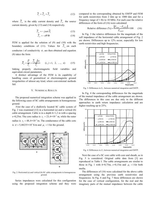
In Fig. 3 the relative differences for the magnitude of the
self impedance of the horizontal cable arrangement of Fig. 2
are shown. Differences up to 12% occur, especially for low
earth resistivities and high frequencies.
difference(%)
40%
30%
20%
10%
ρ=2 Ωm ρ=10 Ωm
ρ=50 Ωm ρ=100 Ωm
ρ=200 Ωm ρ=300 Ωm
ρ=500 Ωm ρ=1000 Ωm
0%
1,E+00 1,E+01 1,E+02 1,E+03 1,E+04 1,E+05 1,E+06 1,E+07
frequency(Hz)
Fig. 3: Differences in Z 11 between numerical integration and EMTP.
In Fig. 4 the corresponding differences for the magnitude
of the mutual impedance of the cable arrangement are shown.
The differences in this case are due only to the different
approaches in earth return impedance calculation and are
higher reaching up to 25%.
difference(%)
40%
30%
20%
10%
ρ=2 Ωm ρ=10 Ωm
ρ=50 Ωm ρ=100 Ωm
ρ=200 Ωm ρ=300 Ωm
ρ=500 Ωm ρ=1000 Ωm
r s
r s
r s
s
a
s
Fig. 2: Horizontal (a) and vertical (b) SC cable arrangements in homogeneous
ground.
Series impedances were calculated for this configuration
using the proposed integration scheme and they were
s
s
b
r s
r c
r c
r s
r s
0%
1,E+00 1,E+01 1,E+02 1,E+03 1,E+04 1,E+05 1,E+06 1,E+07
frequency(Hz)
Fig. 4: Differences in Z 12 between numerical integration and EMTP.
Next the case of a SC core cable with core and sheath, as in
Fig. 5 is considered. Original cable data from [3] are
reproduced in Table I. The cable arrangements are similar to
those in Fig. 1 with h=0,75m, s=0,15m and µ
r
= 1 for both
media.
The differences of (16) were calculated for the above cable
arrangement using the previous earth resistivities and
frequencies. In Fig. 6 and Fig. 7 these differences are shown
for the case of vertical configuration, for the real and the
imaginary parts of the mutual impedance between the cable