Earth Return Path Impedances of Underground Cables for ... - LabPlan
Earth Return Path Impedances of Underground Cables for ... - LabPlan
Earth Return Path Impedances of Underground Cables for ... - LabPlan

Create successful ePaper yourself
Turn your PDF publications into a flip-book with our unique Google optimized e-Paper software.
sheaths respectively. Differences <strong>of</strong> almost 25% are recorded<br />
The results <strong>of</strong> the numerical integration were also checked<br />
against the corresponding by FEM <strong>for</strong> all above cases.<br />
Differences calculated by a <strong>for</strong>mula similar to (16) were less<br />
than 1,5% in all cases over the whole range <strong>of</strong> frequencies<br />
sheath<br />
conductor<br />
r 1<br />
r 2<br />
r 3<br />
r 4<br />
impedance matrices <strong>of</strong> cables buried in a two-layered earth.<br />
The two horizontal arrangements, discussed previously, were<br />
considered.<br />
difference (%)<br />
40%<br />
30%<br />
20%<br />
10%<br />
ρ=2 Ωm ρ=10 Ωm<br />
ρ=50 Ωm ρ=100 Ωm<br />
ρ=200 Ωm ρ=300 Ωm<br />
ρ=500 Ωm ρ=1000 Ωm<br />
.<br />
difference (%)<br />
insulation<br />
Fig. 5: Single Core cable with core and sheath.<br />
Core radius<br />
1<br />
TABLE I.<br />
DATA OF THE SC CABLE OF FIG. 5<br />
Main insulation radius r<br />
2<br />
Sheath radius r<br />
3<br />
Outer insulation radius 4<br />
r 2<br />
Dc resistance <strong>of</strong> copper core<br />
Dc resistance <strong>of</strong> lead sheath<br />
40%<br />
30%<br />
20%<br />
10%<br />
ρ=2 Ωm ρ=10 Ωm<br />
ρ=50 Ωm ρ=100 Ωm<br />
ρ=200 Ωm ρ=300 Ωm<br />
ρ=500 Ωm ρ=1000 Ωm<br />
1, 27 ∗10 − m<br />
2, 28∗10 −2 m<br />
2,54∗10 −2 m<br />
r<br />
2<br />
2,79∗10 − m<br />
0,034 Ω/km<br />
0,436 Ω/km<br />
0%<br />
1,E+00 1,E+01 1,E+02 1,E+03 1,E+04 1,E+05 1,E+06 1,E+07<br />
frequency (Hz)<br />
Fig. 6: Real part <strong>of</strong> the mutual impedance <strong>of</strong> cable sheaths. Differences<br />
between numerical integration and EMTP.<br />
. The numerical integration scheme proved to be absolutely<br />
numerically stable. The computation time <strong>for</strong> the numerical<br />
integration was less than 5s <strong>for</strong> a set <strong>of</strong> 280 resistivity and<br />
frequency combinations using an Intel Pentium IV PC at<br />
1,7 GHz.<br />
The case <strong>of</strong> a multi-layered earth was considered next.<br />
Sunde’s extension [8] refers only to conductors over, or on the<br />
surface <strong>of</strong> a multi-layered earth. For the case <strong>of</strong> underground<br />
conductors no solution <strong>for</strong> the electromagnetic field exists.<br />
There<strong>for</strong>e the FEM was used <strong>for</strong> the calculation <strong>of</strong> the<br />
0%<br />
1,E+00 1,E+01 1,E+02 1,E+03 1,E+04 1,E+05 1,E+06 1,E+07<br />
frequency(Hz)<br />
Fig. 7: Imaginary part <strong>of</strong> the mutual impedance <strong>of</strong> cable sheaths. Differences<br />
between numerical integration and EMTP.<br />
Six different two-layered earth models were investigated,<br />
based on actual grounding parameter measurements [16]. The<br />
corresponding data <strong>for</strong> the resistivities <strong>of</strong> the first ρ 1<br />
and<br />
second ρ<br />
2<br />
layer and <strong>for</strong> the depth d <strong>of</strong> the first layer are<br />
shown in Table II. The second layer is <strong>of</strong> infinite extend.<br />
TABLE II.<br />
TWO-LAYERED EARTH MODELS<br />
ρ 1 (Ωm) ρ 2 (Ωm) d(m)<br />
CASE I 372,729 145,259 2,690<br />
CASE II 246,841 1058,79 2,139<br />
CASE III 57,344 96,714 1,651<br />
CASE IV 494,883 93,663 4,370<br />
CASE V 160,776 34,074 1,848<br />
CASE VI 125,526 1093,08 2,713<br />
Cable impedances obtained from FEM <strong>for</strong> the frequency<br />
range <strong>of</strong> 50 Hz to 1 MHz were compared to the corresponding<br />
from the proposed numerical integration scheme, under the<br />
assumption <strong>of</strong> homogeneous earth. The differences calculated<br />
by a <strong>for</strong>mula similar to (16) are shown in Fig. 8 concerning<br />
the magnitude <strong>of</strong> the mutual impedance between the cable<br />
sheaths <strong>of</strong> the SC cable in Fig. 5. The homogeneous earth<br />
model was assumed to have the resistivity ρ<br />
1<br />
<strong>of</strong> the first earth<br />
layer. Differences <strong>of</strong> up to 40% are encountered, even at<br />
power frequency, especially in cases <strong>of</strong> great divergence<br />
between the resistivities <strong>of</strong> the two layers. The differences<br />
seem to be<br />
minimized near the frequencies, <strong>for</strong> which the penetration<br />
depth p given from (17) approaches the depth <strong>of</strong> the first<br />
layer.<br />
1<br />
p = (17)<br />
π f µσ<br />
0