
Create successful ePaper yourself
Turn your PDF publications into a flip-book with our unique Google optimized e-Paper software.
•<br />
•<br />
•<br />
•<br />
•<br />
•<br />
•<br />
•<br />
•<br />
•<br />
•<br />
•<br />
•<br />
•<br />
•<br />
•<br />
•<br />
•<br />
•<br />
•<br />
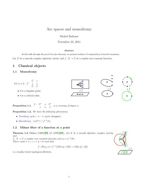
<strong>Arc</strong> <strong>spaces</strong> <strong>and</strong> <strong>monodromy</strong><br />
Michel Raibaut<br />
November 23, 2011<br />
Abstract<br />
In this talk through the proof of a nice theorem, we present technics of computation of motivic measures.<br />
Let X be a smooth complex algebraic variety <strong>and</strong> f : X → C be a regular non constant function.<br />
1 Classical objects<br />
1.1 Monodromy<br />
Let n ≥ 2,<br />
C z<br />
f : ↓ ↓<br />
C z n<br />
• 0 is a singular point.<br />
• 0 is a critical value.<br />
↓ f<br />
•<br />
•<br />
↓ f<br />
↓ f<br />
Proposition 1.1.<br />
f : C ∗ → C ∗<br />
z ↦→ z n is a covering of degree n.<br />
Proposition 1.2. We have the following phenomena<br />
• Vanishing cycles : n−1 cycles disappear .<br />
• Monodromy : π 1 (C ∗ ) f −1 (1).<br />
1.2 Milnor fiber of a function at a point<br />
Theorem 1.3 (Milnor (1968)[12], Lé (1976)[11]). Let X be a smooth algebraic complex variety<br />
<strong>and</strong><br />
f : X → C a regular non constant function <strong>and</strong> x 0 ∈ f −1 (0).<br />
There exists 1 >> ε >> η > 0 such that<br />
x 0<br />
f : B(x 0 ,ε)∩f −1 (D(0,η)\{0}) → D(0,η)\{0}<br />
• •<br />
is a locally trivial topological fibration. 0<br />
↓ f<br />
1
•<br />
•<br />
Definition 1.4. Following this theorem there is two definitions :<br />
1. The Milnor fiber of f at x 0 denoted by F x0 is the fiber of this fibration.<br />
2. The <strong>monodromy</strong> of f at x 0 is the action π 1 (D(0,η)\{0}) F x0 .<br />
The <strong>monodromy</strong> induces a quasi-unipotent operator<br />
T x0 : H ∗ (F x0 ,Q) → H ∗ (F x0 ,Q).<br />
The eigenvalues of this automorphism are roots of unity (<strong>monodromy</strong> theorem).<br />
1.3 Lefschetz numbers of the <strong>monodromy</strong><br />
Definition 1.5. For any natural number n, we consider the Lefschetz numbers<br />
Λ(T n x 0<br />
) := ∑ q≥0(−1) q Trace(T n x 0<br />
,H q (F x0 ,Q))<br />
of the n-th iterate of the <strong>monodromy</strong> T x0 .<br />
Proposition 1.6 (A’Campo (73) [1], A’Campo-Deligne (75)) [2]). Let f : X → C be a regular non constant<br />
morphism on a smooth algebraic variety. We have the following equalities : Λ(T m x 0<br />
) = 0 for 0 < m < µ with µ<br />
the multiplicity of f at x 0 .<br />
2 Lefschetz numbers <strong>and</strong> jet-<strong>spaces</strong><br />
Denef-Loeser in [6] consider for all number n ≥ 1<br />
X n,1 (f) := {ϕ ∈ L n (X) | ϕ(0) = x 0 <strong>and</strong>f(ϕ(t)) = 1.t n modt n+1 }.<br />
Theorem 2.1 (Denef-Loeser (2002) [6], Hrushovski-Loeser (preprint 11/2011) [9]).<br />
For every integer n ≥ 1 : Λ(T n x 0<br />
) = χ c (X n,1 (f)).<br />
Remarks 2.2. Note that :<br />
1. The theorem of A’Campo <strong>and</strong> Deligne is a corollary of this theorem.<br />
0<br />
x 0<br />
↓ f<br />
2. The proof of Denef-Loeser, we are going to present is a comparison of the computation of each part of<br />
this equality on a log-resolution.<br />
3. Hrushovski-Loeser gave a proof without the use of a log-resolution !<br />
4. Let X n = {ϕ ∈ L n (X) | f(ϕ) = acf(ϕ)t n +...<strong>and</strong>ϕ(0) = x 0 }. ThetorusC ∗ actson X n byλ.ϕ(t) = ϕ(λt).<br />
The function angular component acf is a topological locally trivial fibration <strong>and</strong> its fiber is X n,1 .<br />
Proof. Strategy<br />
1. Motivic integration<br />
2. Main idea : stratification of arcs !<br />
where<br />
˜ X n,1 := {ϕ ∈ L(X) | f(ϕ(t)) = 1.t n +...}<br />
µ( ˜ X n,1 ) = [X n,1(f)]<br />
L nd<br />
Y L(Y)\L(E) ⊃ Y n,1 = ⊔ I ⊔ (ki) Y (ki)<br />
h ↓ ↓ h ∞ ↓ ↓<br />
X L(X)\L(f −1 (0)) ⊃ ˜X n,1 = ⊔ I ⊔ (ki) X (ki)<br />
2<br />
1.t n
• h is a log-resolution of (X,f −1 (0)) adapted to x 0 .<br />
• in the following we will forget L(E) <strong>and</strong> L(f −1 (0)) which have measure 0.<br />
• h ∞ is a bijection by properness criterium<br />
3. Computation of µ(Y k ) : Find a Zariski locally trivial fibration !<br />
4. By the change variables formula we compute µ( ˜X k ).<br />
5. By summation we will obtain µ( ˜ X n,1 ) <strong>and</strong> then [X n,1 (f)].<br />
6. A comparison with the A’Campo formula [2] gives Eu c (X n,1 ) = Λ(T n x 0<br />
).<br />
We can start the proof :<br />
1. Motivic measure (cf talks of G.Fichou):<br />
a) We call Grothendieck group denoted by K 0 (Var C ) the group<br />
• generated by the isomorphisms classes [X], for all X algebraic variety,<br />
• with the relations [X] = [F]+[X \[F] for all F closed subset of X.<br />
This group has a unique structure of ring defined by [X]×[Y] := [X ×Y] for all varieties.<br />
We denote by L the class [A 1 ] <strong>and</strong> by M the localization K 0 (Var C )[L −1 ].<br />
b) The main relation : Fiber product.<br />
If π : E → B is a Zariski locally trivial fibration of fiber F then [E] = [B]×[F].<br />
c) Let X be a smooth complex algebraic variety of pure dimension d. A subset A ⊂ L(X) is called<br />
cylindrical or constructible if <strong>and</strong> only if there exists an integer n, <strong>and</strong> a constructible subset of<br />
L n (X) such that A = πn −1(C).<br />
Proposition 2.3. The family of cylindrical objects of L(X) is a Bool Algebra.<br />
By [5][Lemma 4.1] (cf talks of A.Reguera), if A ⊂ L(X) is cylindrical at level n, then the truncation map<br />
π m+1 (A) → π m (A) is a Zariski locally trivial fibration <strong>and</strong><br />
[π m+1 (A)]<br />
[L md ]<br />
= [π n(A)]<br />
[L nd ]<br />
=: µ(A).<br />
This function µ is a measure <strong>and</strong> µ(A) is called motivic measure of A.<br />
In our context, ˜Xn,1 is a cylindrical subset <strong>and</strong> µ( ˜X n,1 ) = [π( ˜X n,1)]<br />
L nd .<br />
2. We consider (Y,E,h) a log-resolution of (X,f −1 (0)) adapted to x 0 namely<br />
(a) h : Y → X is proper morphism with Y smooth,<br />
(b) E = h −1 (f −1 (0)) = ∪ i∈A E i is a normal crossing divisor with irreducible components E i smooth,<br />
(c) h : Y \E → X \f −1 (0) is an isomorphism,<br />
(d) h −1 (x 0 ) = ∪ i∈A(x0)E i .<br />
Notations 2.4. We stratify the normal crossing divisor E = ⊔≠I⊂A E 0 I where E0 I = ∩ i∈IE i \ ∪ j∈J E j .<br />
We denote by N i <strong>and</strong> ν i , the multiplicity of f ◦h <strong>and</strong> Jach against E i so : divJach = ∑ i∈A (ν i −1)E i<br />
<strong>and</strong> div(f ◦h) = ∑ i∈A N i(f)E i .<br />
Let I be a subset of A(x 0 ) non empty, let (k i ) ∈ N ∗I simply denoted by k. We define<br />
⎧<br />
⎫<br />
⎨ ord t ψ ∗ E i = k i , i ∈ I, ⎬<br />
Y k :=<br />
⎩ ψ ∈ L(Y) ord t ψ ∗ E i = k i , i /∈ I,<br />
f ◦h(ψ) = 1.t n ⎭<br />
+....<br />
In particular, the order of each arc in Y k against f ◦h <strong>and</strong> Jac(h) is constant :<br />
∀ψ ∈ Y k , ord t f ◦h = ∑ i∈I<br />
k i N i (f)&ord t Jac(h) = ∑ i∈I(ν i −1)k i<br />
3
3. Computation of µ(Y k )<br />
(a) Y k is a cylindrical subset of L(Y), so µ(Y k ) = [π n (Y k )]/L nd .<br />
(b) We haveto compute [π n (Y k )] <strong>and</strong> for this we will find a Zariskilocally trivial fibration. We only have<br />
local data, so : Let U be an affine subset of Y such that f ◦h |E 0<br />
I ∩U is u× ∏ ı∈I zNi i (f), where for all<br />
i in I, z i is the equation of E i ∩U <strong>and</strong> u is a unit. The divisor E is a normal crossing divisor <strong>and</strong> Y<br />
is smooth so there exists (z i ) i/∈I other coordinates such that (z i ) i∈{1,...,d} is a system of coordinates<br />
on U <strong>and</strong> induces an étale map z : U → A d .<br />
(c) This étale map induces an isomorphism<br />
≃<br />
L n (U) → U × A d L n (A d )<br />
.<br />
ϕ ↦→ (ϕ(0),z(ϕ))<br />
In this way, on the right side we have linearized the problem :<br />
⎛<br />
y ∈ U ∩EI 0 , (a jt kj +∗t kj+1 +...+∗t n ) j∈I<br />
(b j +∗t...+∗t n ) j/∈I<br />
π n (Y k,ϕ(0)∈U∩E 0<br />
I<br />
) ≃<br />
⎜ such that a j ≠ 0,j ∈ I<br />
⎝ z(y) = (0,b)<br />
u(y) ∏ i∈I aNi i = 1<br />
⎞<br />
⎟<br />
⎠<br />
↓ (a,y)<br />
{(a,y) ∈ C ∗I ×E 0 I ∩U | u(y)∏ a Ni<br />
i = 1}<br />
≃<br />
C ∗|I|−1 ×({(a,y) ∈ C ∗ ×E 0 I ∩U | u(y)agcd(Ni)i∈I = 1} =: Ẽ◦ I ∩U)<br />
where the last isomorphism is simply given by a change of coordinates in the torus. We can check<br />
easily that (a,y) is a Zariski trivial fibration of fiber A nd−∑ i∈I ki .<br />
We can glue this construction <strong>and</strong> we obtain :<br />
[π n (Y k )] = [Ẽ0 I ](L−1)|I|−1 L nd−∑ i∈I ki .<br />
4. Let X˜<br />
k be equal h(Y k ), by the change variable formula of Kontsevich [10] <strong>and</strong> Denef-Loeser [5]<br />
∫ ∫<br />
µ(Y k ) = 1dµ X = L −ordt Jach d µY = µ(Y k )L −∑ i∈I (νi−1)ki .<br />
X˜<br />
k Y k<br />
Themainpointistoprovethath : π n (Y k ) → π n (X k )isaZariskilocallytrivialfibrationoffiberA ordt Jach .<br />
We obtain<br />
[π n ( X ˜ k )] = [Ẽ0 I ](L−1)|I|−1 L nd−∑ i∈I kiνi .<br />
5. By additivity<br />
[X n,1 ] =<br />
∑<br />
∅̸=I⊂A(x 0)<br />
[Ẽ0 I](L−1) |I|−1 ∑<br />
∑<br />
(k i ) ∈ N ∗<br />
i k iN i (f) = n<br />
L −∑ i∈I kiνi .<br />
6. If we apply the Euler characteristic with compact support by noting that Eu c (L−1) = 0 then we obtain<br />
∑<br />
Eu c (X n,1 ) = N i (f)Eu c (Ei 0 ) = Λ(Tn x 0<br />
),<br />
i ∈ A(x 0 )<br />
N i (f) | n<br />
because in that case Ẽ0 i is a covering of degree N i(f) of Ei 0 . A’Campo in [2] proved the last equality.<br />
4
3 Motivic Milnor fiber at a point<br />
Denef-Loeser [4] introduced the motivic zeta function of f at x 0<br />
Z f,x0 (T) = ∑ n<br />
µ( ˜ X n,1 )T n ∈ M[[T]].<br />
By the previous part <strong>and</strong> summation of geometrical series, this series is rational !<br />
We denote by<br />
Z f,x0 (T) =<br />
∑<br />
S f,x0 := − lim<br />
T→∞ Z f,x 0<br />
(T) =<br />
∅̸=I⊂A(x 0)[Ẽ0 I](L−1) |I|−1∏ i∈I<br />
∑<br />
∅̸=I⊂A(x 0)<br />
This motive is called the Motivic Milnor fiber of f at x 0 [4].<br />
Remarks 3.1. Some precisions :<br />
L −νi T Ni(f)<br />
1−L −νi T Ni(f).<br />
(−1) |I|−1 [Ẽ0 I ](L−1)|I|−1 ∈ M.<br />
1. Iff hascombinatorial data wecanusethem in orderto classifyarcsinstead ofthe Hironaka’sresolution<br />
of singularities. Non-degenerate polynomial map is treated by Guibert [8] <strong>and</strong> the quasi-ordinary case is<br />
treated by González-Pérez-González-Villa [7].<br />
2. There is also a motivic Milnor fiber in R verifying an A’Campo formula (Comte-Fichou [3]).<br />
3. More generally we can work in the relative equivariant setting with varieties of this type<br />
Z ˆµ → f −1 (0) where the fibers of that structural morphism are invariant under the action.<br />
As an example µ n acts on X n,1 , by λ.ϕ(t) = ϕ(λt) <strong>and</strong> ϕ ↦→ ϕ(0) induces a variety Xn<br />
µn → f −1 (0). We<br />
denote by Mˆµ f −1 (0)<br />
the correspondant Grothendieck ring. In the same way Denef-Loeser define a global<br />
motivic zeta function which is also rational<br />
Z f (T) := ∑ n≥1<br />
[X n (f)]L −nd T n = ∑<br />
∅̸=I≠A[Ẽ0 I ](L−1)|I|−1∏ i∈I<br />
L −νi T Ni(f)<br />
1−L −νi T Ni(f).<br />
The limit S f in Mˆµ f −1 (0) is the analogous of the nearby cycle sheaf of Deligne ψ f(Q X ). For this reason<br />
it’s called motivic nearby cycles. The construction is compatible to the restriction : S f,x0 is the fiber<br />
of S f in x 0 like the cohomology groups of the Milnor fiber F x0 are isomorphic to the cohomology group<br />
of ψ f (Q X ) x0 .<br />
4. The log-canonical threshold lct(X,(f)) = minν i /N i which is the smallest pole of Z f .<br />
5. Monodromy conjecture : If L r is a pole of Z f then there exist x ∈ f −1 (0) such that e 2iπr is an<br />
eigenvalue of the <strong>monodromy</strong> of a Milnor fiber of f at x.<br />
References<br />
[1] Norbert A’Campo. Le nombre de lefschetz d’une monodromie. Indag.Math., 35:113–118, 1973.<br />
[2] Norbert A’Campo. La fonction zêta d’une monodromie. Comment. Math. Helv., 50:233–248, 1975.<br />
[3] G. Comte <strong>and</strong> G. Fichou. Grothendieck ring of semialgebraic formulas <strong>and</strong> motivic real milnor fibres.<br />
arXiv:1111.3181, 2011.<br />
[4] Jan Denef <strong>and</strong> François Loeser. Motivic Igusa zeta functions. J. Algebraic Geom., 7(3):505–537, 1998.<br />
5
[5] Jan Denef <strong>and</strong> François Loeser. Germs of arcs on singular algebraic varieties <strong>and</strong> motivic integration.<br />
Invent. Math., 135(1):201–232, 1999.<br />
[6] Jan Denef <strong>and</strong> François Loeser. Lefschetz numbers of iterates of the <strong>monodromy</strong> <strong>and</strong> truncated arcs.<br />
Topology, 41(5):1031–1040, 2002.<br />
[7] PedroDGonzález Pérez<strong>and</strong> Manuel González Villa. Motivic milnor fiber ofaquasi-ordinaryhypersurface.<br />
1105.2480.<br />
[8] Gil Guibert. E<strong>spaces</strong> d’arcs et invariants d’Alex<strong>and</strong>er. Comment. Math. Helv., 77(4):783–820, 2002.<br />
[9] E. Hrushovski <strong>and</strong> F. Loeser. Monodromy <strong>and</strong> the lefschetz fixed point formula. arXiv:1111.1954, 2011.<br />
[10] Kontsevich. Lecture at orsay. Décembre 7, 1995.<br />
[11] Dung Trang Le. Some remarks on relative <strong>monodromy</strong>. In Real <strong>and</strong> complex singularities (Proc. Ninth<br />
Nordic Summer School/NAVF Sympos. Math., Oslo, 1976), pages397–403.Sijthoff <strong>and</strong> Noordhoff, Alphen<br />
aan den Rijn, 1977.<br />
[12] John Milnor. Singular points of complex hypersurfaces. Ann. of math. Studies, Princeton Univ.Press,<br />
Princeton, 61, 1968.<br />
6