A Stub Matched Lazy H for 17 M Introduction The author has ...

A Stub Matched Lazy H for 17 M
Introduction
The author has experimented with various configurations of the classic Lazy H
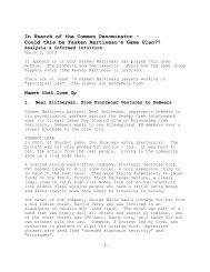
antenna and a version optimised for operation on the 17 M band is shown in Figure 1.
The antenna conductors are 14 SWG seven strand copper, and all transmission lines
and the stub are constructed from 450 ohm window line.
29 ft.
50 ft. agl
450 ohm
transposed
20 ft. 25 ft.
25 ft. agl
14 ft. 2"
all transmission lines
450 "window"
450 ohm
TL to rig
approx. 160 ft.
3 ft. 4"
s/c stub
Figure 1 – Lazy H Dimensions
Note that the stub method of matching described here is inherently narrowband, and
prevents the antenna being used effectively on other bands, particularly 7 MHz, 14
MHz and 21 MHz, where it can still produce useful radiation patterns. If this is a
concern, then it is preferable to just accept the slight loss of gain and trickier tuning
with the unmatched configuration. If the transmission line run is relatively short, say
less than 50 ft., then this should not be a problem in practice, but with longer runs the
losses can be quite significant if the SWR on the 450 ohm line is already high, and the
matching can be very susceptible to water or wet snow on the line. In my installation
the transmission line was required to be around 175 ft. in length so I decided to install
a stub at the antenna to match the antenna impedance to the 450 ohm transmission
line impedance over the 17 M band.
Antenna Pattern and SWR Plots
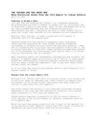
Figure 2 shows the elevation radiation pattern of the Lazy H over medium ground.
Maximum gain is 12.3 dBi at an elevation angle of 18 degrees. At 5 degrees the gain
is still a respectable 5.4 dBi. The patterns are independent of the stub match since the
model assumes zero transmission line and mismatch loss.

Figure 2 – Elevation Radiation Pattern
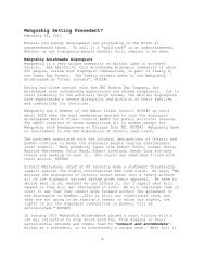
The corresponding azimuth pattern at 18 degrees take off angle is shown in Figure 3.
Figure 3 – Azimuth Radiation Pattern
The azimuth pattern maxima are at right angles to the plane of the antenna, or NE /
SW as installed at the author’s QTH in eastern Ontario.
Figure 4 shows the antenna SWR into 450 ohms, without stub matching and plotted
from 15 to 20 MHz.

Figure 4 – Unmatched 15 to 20 MHz VSWR
At 18.14 MHz the SWR is 6.4:1, with Z 0 = 277 + j734. Variation over the band is
insignificant. The antenna therefore presents a fairly high inductive reactance
loading, but with a reasonably well-matched resistive component.
Line Losses and SWR
The SWR measured by a 450 ohm balanced bridge at the transmitter end of the line,
before matching and in dry weather, was 6.5:1 at 18.14 MHz, or close to the model
value. A repeat check made when the feeder was wet due to moderate rain gave a
measured SWR of around 4. The rain also required retuning of the Z match tuner
usually used to match the antenna feed line to the 50 ohm unbalanced transceiver RF
port.
The loss due to 175 ft. of 450 ohm transmission line between the tuner and the centre
of the lower element of the antenna was estimated at 0.12 dB / 100 ft. from the chart
(Fig. 19.4) in the ARRL Handbook (1999). Applying the formulae shown below
gives the actual loss (around 0.5 dB) for 175 ft. of line operating at 6.5:1 SWR.
This may not appear to be a particularly significant loss; however the calculation
assumes dry transmission line under ideal conditions. In wet weather the line losses
almost certainly increase, and there is the additional inconvenience of having to reset
the antenna tuner.

Matched line loss:
SWR at load:
ML := .12
ML
10
a := 10
SWR := 6.5
dB per 100 ft. from ARRL HB pp.19.5
ρ :=
SWR − 1
SWR + 2
Mismatched line loss:
Measured line length:
MML := 10⋅log
MML = 0.285
L := 175
MML = 0.499
a 2 − ρ 2
a⋅
1 − ρ
ft.
dB
( ) 2
MML :=
L⋅
MML
100
dB per 100ft.
Matching Stub Calculations
The first step is to calculate the position of the first current maximum on the
transmission line, working from the antenna. In the absence of a suitable current
probe, the best method is to work in from the outer end of the antenna elements to
find the position of the first current maximum on the transmission line. At this point
the impedance on the line consists of a real resistive component equal to the
characteristic impedance of the line in parallel with a reactive component.
In this case the length of one of the lower elements (29 ft.) is 0.53 λ, where λ = 54.22
ft.. Since the element length is of the order of ½ λ, the next accessible current
maximum occurs at ¾ λ from the outer end of the element, or at L = 0.25 – 0.03 =
0.22 λ along the transmission line from its junction with that element. Taking the
velocity factor of the line into account, L is given by: L = 54.22 x 0.22 x 0.95 = 11.33
ft. In the case of the upper set of elements, also 0.53λ in length, there is an additional
20 ft. of phasing line to take into account. Ideally the length of this line should be
0.5λ or 25.75 ft, accounting for the 0.95 velocity factor, in which case the current
maximum due to the upper elements would coincide with the position of the
maximum due to the lower elements. However a shorter phasing line length of 20 ft.
is used in the antenna described here because it allows tension to be maintained in the
phasing line and, according to the model, the shorter phasing line actually improves
the gain by a few 10ths of a dB (attempts to use the ideal 25.75 ft. length with 25 ft.
vertical support halyard spacing resulted in excessive thrashing under high wind
conditions and broken phasing line connections). The current maximum for the upper
elements thus occurs at 5.75 ft. closer to the transmitter than that for the lower
elements. A compromise stub position of 11.33 + 5.75/2 = 14.2 ft. (14 ft. 2”) is
therefore indicated.
The next step is to find the required length of a short circuit stub to connect at the
current maximum to in order to compensate for the antenna’s reactive impedance.
The procedure is to draw a circle on the Smith chart as shown in Figure 5,
corresponding to the measured 6.5:1 SWR and centred on R/Z 0 = 1. This circle
crosses the unit resistance circle at a point corresponding to an inductive reactance of
j2.3. Follow the j2.3 curve to the edge of the chart and note the reading on the

wavelength scale. Then calculate the total length in wavelengths from this point to
the infinite susceptance (short circuit) point on the right of the horizontal axis. In this
example the j2.3 curve intersects the 0.185λ point on the outer scale, and the
difference between this value and 0.25λ, corresponding to infinite susceptance, is
0.065λ, or 54.22 x 0.95 = 3.34 ft (3 ft. 4”).
Figure 5 – Smith Chart
A short circuit stub was made from 450 ohm line to the above length and attached in
parallel with the transmission line at the previously calculated position of the current
maximum (14 ft. 2”). The measured SWR improved to 1.2:1 at the center of the 18
MHz band, with negligible variation over the band. If necessary the SWR can be
optimized by adjusting the stub dimensions after observing the frequency at which
minimum SWR is obtained. For example if this frequency is higher than the desired
operating frequency by X%, then the stub spacing from the antenna feed point and
stub length can be increased by 0.95X%. In practice it appears that stub position is
the more critical dimension so try this first.
The stub match was found to considerably reduce environmental detuning effects. An
additional benefit is that the stub provides a DC short circuit across an otherwise open
circuit antenna thereby reducing the chances of static build up and allowing for
straightforward ohm-meter transmission line continuity checks.
Nick Shepherd VE3OWV