Solving log-determinant optimization problems by a Newton-CG ...

Solving log-determinant optimization
problems by a Newton-CG primal proximal
point algorithm
Chengjing Wang ∗ , Defeng Sun † and Kim-Chuan Toh ‡
September 29, 2009
Abstract
We propose a Newton-CG primal proximal point algorithm for solving large
scale log-determinant optimization problems. Our algorithm employs the essential
ideas of the proximal point algorithm, the Newton method and the preconditioned
conjugate gradient solver. When applying the Newton method to solve the inner
sub-problem, we find that the log-determinant term plays the role of a smoothing
term as in the traditional smoothing Newton technique. Focusing on the problem
of maximum likelihood sparse estimation of a Gaussian graphical model, we
demonstrate that our algorithm performs favorably comparing to the existing stateof-the-art
algorithms and is much more preferred when a high quality solution is
required for problems with many equality constraints.
Keywords: Log-determinant optimization problem, Sparse inverse covariance selection,
Proximal-point algorithm, Newton’s method
1 Introduction
In this paper, we consider the following standard primal and dual log-determinant (logdet)
problems:
(P ) min{〈C, X〉 − µ log det X : A(X) = b, X ≻ 0},
X
(D)
max
y,Z {bT y + µ log det Z + nµ(1 − log µ) : Z + A T y = C, Z ≻ 0},
∗ Singapore-MIT Alliance, 4 Engineering Drive 3, Singapore 117576 (smawc@nus.edu.sg).
† Department of Mathematics and NUS Risk Management Institute, National University of Singapore,
2 Science Drive 2, Singapore 117543 (matsundf@nus.edu.sg). The research of this author is partially
supported by the Academic Research Fund Under Grant R-146-000-104-112.
‡ Department of Mathematics, National University of Singapore, 2 Science Drive 2, Singapore 117543
(mattohkc@nus.edu.sg); and Singapore-MIT Alliance, 4 Engineering Drive 3, Singapore 117576.
1

where S n is the linear space of n × n symmetric matrices, C ∈ S n , b ∈ R m , µ ≥ 0 is
a given parameter, and 〈·, ·〉 stands for the standard trace inner product in S n . Here
A : S n → R m is a linear map and A T : R m → S n is the adjoint of A. We assume that
A is surjective, and hence AA T is nonsingular. The notation X ≻ 0 means that X is a
symmetric positive definite matrix. We further let S n + (resp., S n ++) to be the cone of n × n
symmetric positive semidefinite (resp., definite) matrices. Note that the linear maps A
and A T can be expressed, respectively, as
A(X) =
[
〈A 1 , X〉, . . . , 〈A m , X〉] T
, A T (y) =
m∑
y k A k ,
where A k , k = 1, · · · , m are given matrices in S n .
It is clear that the log-det problem (P ) is a convex optimization problem, i.e., the
objective function 〈C, X〉 − µ log det X is convex (on S n ++), and the feasible region is
convex. The log-det problems (P ) and (D) can be considered as a generalization of linear
semidefinite programming (SDP) problems. One can see that in the limiting case where
µ = 0, they reduce, respectively, to the standard primal and dual linear SDP problems.
Log-det problems arise in many practical applications such as computational geometry,
statistics, system identification, experiment design, and information and communication
theory. Thus the algorithms we develop here can potentially find wide applications. One
may refer to [5, 24, 21] for an extensive account of applications of the log-det problem.
For small and medium sized log-det problems, including linear SDP problems, it is
widely accepted that interior-point methods (IPMs) with direct solvers are generally very
efficient and robust; see for example [21, 22]. For log-det problems with m large and n
moderate (say no more than 2, 000), the limitations faced by IPMs with direct solvers
become very severe due to the need of computing, storing, and factorizing the m × m
Schur matrices that are typically dense.
Recently, Zhao, Sun and Toh [28] proposed a Newton-CG augmented Lagrangian
(NAL) method for solving linear SDP problems. This method can be very efficient when
the problems are primal and dual nondegenerate. The NAL method is essentially a proximal
point method applied to the primal problem where the inner sub-problems are solved
by an inexact semi-smooth Newton method using a preconditioned conjugate gradient
(PCG) solver. Recent studies conducted by Sun, Sun and Zhang [20] and Chan and Sun
[6] revealed that under the constraint nondegenerate conditions for (P ) and (D) (i.e.,
the primal and dual nondegeneracy conditions in the IPMs literature, e.g., [1]), the NAL
method can locally be regarded as an approximate generalized Newton method applied
to a semismooth equation. The latter result may explain to a large extent why the NAL
method can be very efficient.
As the log-det problem (P ) is an extension of the primal linear SDP, it is natural for
us to further use the NAL method developed for linear SDPs to solve log-det problems.
Following what has been done in linear SDPs, our approach is to apply a Newton-CG
primal proximal point algorithm (PPA) to (1), and then to use an inexact Newton method
2
k=1

to solve the inner sub-problems by using a PCG solver to compute inexact Newton directions.
We note that when solving the inner sub-problems in the NAL method for linear
SDPs [28], a semi-smooth Newton method has to be used since the objective functions
are differentiable but not twice continuously differentiable. But for log-det problems, the
objective functions in the inner sub-problems are twice continuously differentiable (actually,
analytic) due to the fact that the term −µ log det X acts as a smoothing term. This
interesting phenomenon implies that the standard Newton method can be used to solve
the inner sub-problem. It also reveals a close connection between adding the log-barrier
term −µlog detX to a linear SDP and the technique of smoothing the KKT conditions
[6].
In [18, 19], Rockafellar established a general theory on the global convergence and
local linear rate of convergence of the sequence generated by the proximal point and
augmented Lagrangian methods for solving convex optimization problems including (P )
and (D). Borrowing Rockafellar’s results, we can establish global convergence and local
convergence rate for our Newton-CG PPA method for (P ) and (D) without much difficulty.
In problem (P ), we only deal with a matrix variable, but the PPA method we develop
in this paper can easily be extended to the following more general log-det problems to
include vector variables:
min{〈C, X〉 − µ log det X + c T x − ν log x : A(X) + Bx = b, X ≻ 0, x > 0}, (1)
max{b T y + µ log det Z + ν log z + κ : Z + A T y = C, z + B T y = c, Z ≻ 0, z > 0}, (2)
where ν > 0 is a given parameter, c ∈ R l and B ∈ R m×l are given data, and κ =
nµ(1 − log µ) + lν(1 − log ν).
In the implementation of our Newton-CG PPA method, we focus on the maximum
likelihood sparse estimation of a Gaussian graphical model (GGM). This class of problems
includes two subclasses. The first subclass is that the conditional independence of a model
is completely known, and it can be formulated as follows:
min
X
{
〈S, X〉 − log detX : X ij = 0, ∀ (i, j) ∈ Ω, X ≻ 0
}
, (3)
where Ω is the set of pairs of nodes (i, j) in a graph that are connected by an edge,
and S ∈ S n is a given sample covariance matrix. Problem (3) is also known as a sparse
covariance selection problem. In [7], Dahl, Vandenberghe and Roychowdhury showed
that when the underlying dependency graph is nearly-chordal, an inexact Newton method
combined with an appropriate PCG solver can be quite efficient in solving (3) with n up
to 2, 000 but on very sparse data (for instance, when n = 2, 000, the number of upper
nonzeros is only about 4, 000 ∼ 6, 000). But for general large scale problems of the form
(3), little research has been done in finding efficient algorithms to solve the problems. The
second subclass of the GGM is that the conditional independence of the model is partially
known, and it is formulated as follows:
min
{〈S, X〉 − log det X + ∑
}
ρ ij |X ij | : X ij = 0, ∀ (i, j) ∈ Ω, X ≻ 0 . (4)
X
(i,j)∉Ω
3

In [8], d’Aspremont, Banerjee, and El Ghaoui, among the earliest, proposed to apply
Nesterov’s smooth approximation (NSA) scheme to solve (4) for the case where Ω = ∅.
Subsequently, Lu [10, 11] suggested an adaptive Nesterov’s smooth (ANS) method to
solve (4). The ANS method is currently one of the most effective methods for solving
large scale problems (e.g., n ≥ 1, 000, m ≥ 500, 000) of the form (4). In the ANS method,
the equality constraints in (4) are removed and included in the objective function via
the penalty approach. The main idea in the ANS method is basically to apply a variant
of Nesterov’s smooth method [16] to solve the penalized problem subject to the single
constraint X ≻ 0. In fact, both the ANS and NSA methods have the same principle
idea, but the latter runs much slowly than the former. In contrast to IPMs, the greatest
merit of the ANS method is that it needs much lower storage and computational cost per
iteration. In [10], the ANS method has been demonstrated to be rather efficient in solving
randomly generated problems of form (4), while obtaining solutions with low/moderate
accuracy. However, as the ANS is a first-order method, it may require huge computing
cost to obtain high accuracy solutions. In addition, as the penalty approach is used in the
ANS method to solve (4), the number of iterations may increase drastically if the penalty
parameter is updated frequently. Another limitation of the ANS method introduced in
[10] is that it can only deal with the special equality constraints in (4). It appears to be
difficult to extend the ANS method to deal with more general equality constraints of the
form A(X) = b.
Our numerical results show that for both problems (3) and (4), our Newton-CG PPA
method can be very efficient and robust in solving large scale problems generated as in
[8] and [10]. Indeed, we are able to solve sparse covariance selection problems with n
up to 2, 000 and m up to 1.8 × 10 6 in about 54 minutes. For problem (4), our method
consistently outperforms the ANS method by a substantial margin, especially when the
problems are large and the required accuracy tolerances are relatively high.
The remaining part of this paper is organized as follows. In Section 2, we give some
preliminaries including a brief introduction on concepts related to the proximal point
algorithm. In Section 3 and 4, we present the details of the PPA method and Newton-
CG algorithm. In Section 5, we give the convergence analysis of our PPA method. The
numerical performance of our algorithm is presented in Section 6. Finally, we give some
concluding remarks in Section 7.
2 Preliminaries
For the sake of subsequent discussions, we first introduce some concepts related to the
proximal point method based on the classic papers by Rockafellar [18, 19].
Let H be a real Hilbert space with an inner product 〈·, ·〉. A multifunction T : H ⇒ H
is said to be a monotone operator if
〈z − z ′ , w − w ′ 〉 ≥ 0, whenever w ∈ T (z), w ′ ∈ T (z ′ ). (5)
4

It is said to be maximal monotone if, in addition, the graph
G(T ) = {(z, w) ∈ H × H| w ∈ T (z)}
is not properly contained in the graph of any other monotone operator T ′ : H ⇒ H.
For example, if T is the subdifferential ∂f of a lower semicontinuous convex function
f : H → (−∞, +∞], f ≢ +∞, then T is maximal monotone (see Minty [13] or Moreau
[14]), and the relation 0 ∈ T (z) means that f(z) = min f.
Rockafellar [18] studied a fundamental algorithm for solving
0 ∈ T (z), (6)
in the case of an arbitrary maximal monotone operator T . The operator P = (I + λT ) −1
is known to be single-valued from all of H into H, where λ > 0 is a given parameter. It
is also nonexpansive:
‖P (z) − P (z ′ )‖ ≤ ‖z − z ′ ‖,
and one has P (z) = z if and only if 0 ∈ T (z). The operator P is called the proximal
mapping associate with λT , following the terminology of Moreau [14] for the case of
T = ∂f.
The PPA generates, for any starting point z 0 , a sequence {z k } in H by the approximate
rule:
z k+1 ≈ (I + λ k T ) −1 (z k ).
Here {λ k } is a sequence of positive real numbers. In the case of T = ∂f, this procedure
reduces to
{
z k+1 ≈ arg min f(z) + 1 }
‖z − z k ‖ 2 . (7)
z 2λ k
Definition 2.1. (cf. [18]) For a maximal monotone operator T , we say that its inverse
T −1 is Lipschitz continuous at the origin (with modulus a ≥ 0) if there is a unique solution
¯z to z = T −1 (0), and for some τ > 0 we have
‖z − ¯z‖ ≤ a‖w‖, where z ∈ T −1 (w) and ‖w‖ ≤ τ.
We state the following lemma which will be needed later in the derivation of the PPA
method for solving (P ).
Lemma 2.1. Let Y be an n × n symmetric matrix with eigenvalue decomposition Y =
P DP T with D = diag(d). We assume that d 1 ≥ · · · ≥ d r > 0 ≥ d r+1 · · · ≥ d n . Let
γ > 0 be given. For the two scalar functions φ + γ (x) := ( √ x 2 + 4γ + x)/2 and φ − γ (x) :=
( √ x 2 + 4γ − x)/2 for all x ∈ R, we define their matrix counterparts:
Y 1 = φ + γ (Y ) := P diag(φ + γ (d))P T and Y 2 = φ − γ (Y ) := P diag(φ − γ (d))P T . (8)
5

Then
(a) The following decomposition holds: Y = Y 1 − Y 2 , where Y 1 , Y 2 ≻ 0, and Y 1 Y 2 = γI.
(b) φ + γ is continuously differentiable everywhere in S n and its derivative (φ + γ ) ′ (Y )[H] at
Y for any H ∈ S n is given by
where Ω ∈ S n is defined by
(φ + γ ) ′ (Y )[H] = P (Ω ◦ (P T HP ))P T ,
Ω ij =
φ + γ (d i ) + φ + γ (d j )
√
d
2
i + 4γ +
√d 2 j + 4γ , i, j = 1, . . . , n.
(c) (φ + γ ) ′ (Y )[Y 1 + Y 2 ] = φ + γ (Y ).
Proof. (a) It is easy to verify that the decomposition holds. (b) The result follows from
[3, Ch. V.3.3] and the fact that
φ + γ (d i ) − φ + γ (d j )
d i − d j
=
φ + γ (d i ) + φ + γ (d j )
√
d
2
i + 4γ +
√d 2 j + 4γ , d i ≠ d j .
(
)
(c) We have (φ + γ ) ′ (Y )[Y 1 + Y 2 ] = P Ω ◦ diag(φ + γ (d) + φ − γ (d)) P T = P diag(φ + γ (d))P T ,
and the required result follows.
3 The primal proximal point algorithm
Define the feasible sets of (P ) and (D), respectively, by
F P = {X ∈ S n : A(X) = b, X ≻ 0}, F D = {(y, Z) ∈ R m × S n : Z + A T y = C, Z ≻ 0}.
Throughout this paper, we assume that the following conditions for (P ) and (D) hold.
Assumption 3.1. Problem (P ) satisfies the condition
∃ X 0 ∈ S++ n such that A(X 0 ) = b. (9)
Assumption 3.2. Problem (D) satisfies the condition
∃ (y 0 , Z 0 ) ∈ R m × S++ n such that Z 0 + A T y 0 = C. (10)
6

Under the above assumptions, problem (P ) has a unique optimal solution, denoted
by X and problem (D) has a unique optimal solution, denoted by (y, Z). In addition,
the following Karush-Kuhn-Tucker (KKT) conditions are necessary and sufficient for the
optimality of (P ) and (D):
A(X) − b = 0,
Z + A T y − C = 0, (11)
XZ = µI, X ≻ 0, Z ≻ 0.
The last condition in (11) can be easily seen to be equivalent to the following condition
φ + γ (X − λZ) = X with γ := λµ (12)
for any given λ > 0, where φ + γ is defined by (8) in Lemma 2.1. Recall that for the linear
SDP case (where µ = 0), the complementarity condition XZ = 0 with X, Z ≽ 0, is
equivalent to Π + (X − λZ) = X, for any λ > 0, where Π + (·) is the metric projector
onto S+. n One can see from (12) that when µ > 0, the log-barrier term µlog detX in (P )
contributed to a smoothing term in the projector Π + .
Lemma 3.1. Given any Y ∈ S n and λ > 0, we have
{ 1
}
min
Z≻0 2λ ‖Y − Z‖2 − µ log det Z = 1
2λ ‖φ− γ (Y )‖ 2 − µ log det(φ + γ (Y )), (13)
where γ = λµ.
Proof. Note that the minimization problem in (13) is an unconstrained problem and the
objective function is strictly convex and continuously differentiable. Thus any stationary
point would be the unique minimizer of the problem. The stationary point, if it exists, is
the solution of the following equation:
Y = Z − γZ −1 . (14)
By Lemma 2.1(a), we see that Z ∗ := φ + γ (Y ) satisfies (14). Thus the optimization problem
in (13) has a unique minimizer and the minimum objective function value is given by
1
2λ ‖Y − Z ∗‖ 2 − µ log det Z ∗ = 1
2λ ‖φ− γ (Y )‖ 2 − µ log det(φ + γ (Y )).
This completes the proof.
By defining log 0 := −∞, we can see that problems (P ) and (D) are equivalent to
(P ′ ) min{〈C, X〉 − µ log det X : A(X) = b, X ≽ 0},
X
(D ′ ) max
y,Z {bT y + µ log det Z : Z + A T y = C, Z ≽ 0}.
7

Due to this equivalence, from now on we focus on (P ′ ) and (D ′ ), rather on (P ) and (D).
Let l(X; y) : S n × R m → R be the ordinary Lagrangian function for (P ) in extended
form:
{
〈C, X〉 − µ log det X + 〈y, b − A(X)〉 if X ∈ S
n
+ ,
l(X; y) =
(15)
∞
otherwise.
The essential objective function in (P ′ ) is given by
{
〈C, X〉 − µ log det X if X ∈
f(X) = max l(X; y) = FP ,
y∈R m ∞
otherwise.
For later developments, we define the following maximal monotone operator associated
with l(X, y):
T l (X, y) := {(U, v) ∈ S n × R m | (U, −v) ∈ ∂l(X, y), (X, y) ∈ S n × R m }.
Let F λ be the Moreau-Yosida regularization (see [14, 27]) of f in (16) associated with
λ > 0, i.e.,
F λ (X) = min
Y ∈S n{f(Y ) + 1
2λ ‖Y − X‖2 } = min {f(Y ) + 1
Y ∈S++
n 2λ ‖Y − X‖2 }. (17)
From (16), we have
where
F λ (X) = min
Θ λ (X, y) = min
Y ∈S n ++
{
sup
Y ∈S++
n y∈R m
= sup
min
y∈R m Y ∈S++
n
l(Y ; y) + 1 }
2λ ‖Y − X‖2
{
l(Y ; y) + 1 }
2λ ‖Y − X‖2
{
l(Y ; y) + 1
2λ ‖Y − X‖2 }
{
= b T y + min 〈C − A T y, Y 〉 − µlog detY + 1
Y ∈S++
n
2λ ‖Y − X‖2 }
(16)
= sup
y∈R m Θ λ (X, y) , (18)
= b T y − 1
2λ ‖W λ(X, y)‖ 2 + 1
{ 1
2λ ‖X‖2 + min
Y ∈S++
n 2λ ‖Y − W λ(X, y)‖ 2 − µlog detY
Here W λ (X, y) := X − λ(C − A T y). Note that the interchange of min and sup in (18)
follows from [17, Theorem 37.3]. By Lemma 3.1, the minimum objective value in the
above minimization problem is attained at Y ∗ = φ + γ (W λ (X, y)). Thus we have
Θ λ (X, y) = b T y + 1
2λ ‖X‖2 − 1
2λ ‖φ+ γ (W λ (X, y))‖ 2 − µlog det φ + γ (W λ (X, y)) + nµ. (19)
Note that for a given X, the function Θ(X, ·) is analytic, cf. [23]. Its first and second
order derivatives can be computed as in the following lemma.
8
}
.

Lemma 3.2. For any y ∈ R m and X ≻ 0, we have
∇ y Θ λ (X, y) = b − Aφ + γ (W λ (X, y)) (20)
∇ 2 yyΘ λ (X, y) = −λA(φ + γ ) ′ (W λ (X, y))A T (21)
Proof. To simplify notation, we use W to denote W λ (X, y) in this proof. To prove (20),
note that
∇ y Θ(X, y) = b − A(φ + γ ) ′ (W )[φ + γ (W )] − λµA(φ + γ ) ′ (W )[(φ + γ (W )) −1 ]
= b − A(φ + γ ) ′ (W )[φ + γ (W ) + φ − γ (W )].
By Lemma 2.1(c), the required result follows. From (20), the result in (21) follows readily.
Let y λ (X) be such that
y λ (X) ∈ arg sup
y∈R m Θ λ (X, y).
Conse-
Then we know that φ + γ (W (X, y λ (X))) is the unique optimal solution to (17).
quently, we have that F λ (X) = Θ λ (X, y λ (X)) and
∇F λ (X) = 1 λ
(
)
X − φ + γ (W (X, y λ (X))) = C − A T y − 1 λ φ− γ (W (X, y λ (X))). (22)
Given X 0 ∈ S n ++, the exact PPA for solving (P ′ ), and thus (P ), is given by
X k+1
{
= (I + λ k T f ) −1 (X k ) = arg min f(X) + 1
}
‖X − X k ‖ 2 , (23)
X∈S++
n 2λ k
where T f = ∂f. It can be shown that
X k+1 = X k − λ k ∇F λk (X k ) = φ + γ k
(W (X k , y λk (X k ))), (24)
where γ k = λ k µ.
The exact PPA outlined in (23) is impractical for computational purpose. Hence we
consider an inexact PPA for solving (P ′ ), which has the following template.
9

Algorithm 1: The Primal PPA. Given a tolerance ε > 0. Input X 0 ∈ S n ++ and λ 0 > 0.
Set k := 0. Iterate:
Step 1. Find an approximate maximizer
{
}
y k+1 ≈ arg sup θ k (y) := Θ λk (X k , y) , (25)
y∈R m
where Θ λk (X k , y) is defined as in (19).
Step 2. Compute
X k+1 = φ + γ k
(W λk (X k , y k+1 )), Z k+1 = 1 λ k
φ − γ k
(W λk (X k , y k+1 )). (26)
Step 3. If ‖R k+1
d
:= (X k − X k+1 )/λ k ‖ ≤ ɛ; stop; else; update λ k ; end.
Remark 3.1. Note that b−A(X k+1 ) = b−Aφ + γ k
(W λk (X k , y k+1 )) = ∇ y Θ λk (X k , y k+1 ) ≈ 0.
Remark 3.2. Observe that the function Θ λ (X, y) is twice continuously differentiable (actually,
analytic) in y. In contrast, its counterpart L σ (y, X) for a linear SDP in [28] fails
to be twice continuously differentiable in y and only the Clarke’s generalized Jacobian of
∇ y L σ (y, X) (i.e., ∂∇ y L σ (y, X)) can be obtained. This difference can be attributed to the
term −µ log det X in problem (P ′ ). In other words, −µ log det X works as a smoothing
term that turns L σ (y, X) (which is not twice continuously differentiable) into an analytic
function in y. This idea is different from the traditional smoothing technique of using
a smoothing function on the KKT conditions since the latter is not motivated by adding
a smoothing term to an objective function. Our derivation of Θ λ (y, X) shows that the
smoothing technique of using a squared smoothing function φ + γ (x) = ( √ x 2 + 4γ + x)/2
can indeed be derived by adding the log-barrier term to the objective function.
The advantage of viewing the smoothing technique from the perspective of adding a
log-barrier term is that the error between the minimum objective function values of the
perturbed problem and the original problem can be estimated. In the traditional smoothing
technique for the KKT conditions, there is no obvious mean to estimate the error in
the objective function value of the solution computed from the smoothed KKT conditions
from the true minimum objective function value. We believe the connection we discovered
here could be useful for the error analysis of the smoothing technique applied to the KKT
conditions.
For the sake of subsequent convergence analysis, we present the following proposition.
Proposition 3.1. Suppose that (P ′ ) satisfies (9). Let X ∈ S++ n be the unique optimal
solution to (P ′ ), i.e., X = T −1
f
(0). Then T −1 is Lipschitz continuous at the origin.
f
10

Proof. From [19, Prop. 3], it suffices to show that the following quadratic growth condition
holds at ¯X for some positive constant α:
f(X) ≥ f(X) + α‖X − X‖ 2 ∀ X ∈ N such that X ∈ F P (27)
where N is a neighborhood of X in S n ++. From [4, Theorem 3.137], to prove (27), it
suffices to show the second order sufficient condition for (P ′ ) holds.
Now for X ∈ S n ++, we have
〈∆X, ∇ 2 XXl(X; y)(∆X)〉 = µ〈X −1 ∆XX −1 , ∆X〉 ≥ µλ −2
max(X)‖∆X‖ 2 , ∀ ∆X ∈ S n ,
where λ max (X) is the maximal eigenvalue of X, this is equivalent to
〈∆X, ∇ 2 XXl(X; y)(∆X)〉 > 0, ∀ ∆X ∈ S n \ {0}. (28)
Certainly, (28) implies the second order sufficient condition for Problem (P ′ ).
We can also prove in parallel that the maximal monotone operator T l is Lipschitz
continuous at the origin.
4 The Newton-CG method for inner problems
In the algorithm framework proposed in Section 3, we have to compute y k+1 ≈ argmax
{θ k (y) : y ∈ R m }. In this paper, we will introduce the Newton-CG method to achieve
this goal.
11

Algorithm 2: The Newton-CG Method.
Step 0. Given µ ∈ (0, 1 2 ), ¯η ∈ (0, 1), τ ∈ (0, 1], τ 1, τ 2 ∈ (0, 1), and δ ∈ (0, 1), choose
y 0 ∈ R m .
Step 1. For k = 0, 1, 2, . . . ,
Step 1.1. Given a maximum number of CG iterations n j > 0 and compute.
η j := min{¯η, ‖∇ y θ k (y j )‖ 1+τ }.
Apply the CG method to find an approximate solution d j to
(∇ 2 yyθ k (y j ) + ɛ j I)d = −∇ y θ k (y j ), (29)
where ɛ j := τ 1 min{τ 2 , ‖∇ y θ k (y j )‖}.
Step 1.2. Set α j = δ m j
, where m j is the first nonnegative integer m for which
Step 1.3. Set y j+1 = y j + α j d j .
θ k (y j + δ m d j ) ≥ θ k (y j ) + µδ m 〈∇ y θ k (y j ), d j 〉.
From (21) and the positive definiteness property of φ ′ +(W (y; X)) (for some properties
of the projection operator one may refer to [12]), we have that −∇ 2 yyθ k (y j ) is always
positive definite, then −∇ 2 yyθ k (y j ) + ɛ j I is positive definite as long as ∇ y θ k (y j ) ≠ 0. So
we can always apply the PCG method to (29). Of course, the direction d j generated from
(29) is always an ascent direction. With respect to the analysis of the global convergence
and local quadratic convergence rate of the above algorithm, we will not present the
details, and one may refer to Section 3.3 of [28] since it is very similar to the semismooth
Newton-CG algorithm used in that paper. The difference lies in that d j obtained from
(29) in this paper is an approximate Newton direction; in contrast, d j obtained from (62)
in [28] is an approximate semimsooth Newton direction.
5 Convergence analysis
Global convergence and the local convergence rate of our Newton-CG PPA method to
problems (P ′ ) and (D ′ ) can directly be derived from Rockafellar [18, 19] without much
difficulty. For the sake of completeness, we shall only state the results below.
Since we cannot solve the inner problems exactly, we will use the following stopping
12

criteria considered by Rockafellar [18, 19] for terminating Algorithm 2:
(A) sup θ k (y) − θ k (y k+1 ) ≤ ɛ 2 k/2λ k , ɛ k ≥ 0,
∞∑
ɛ k < ∞;
k=0
(B) sup θ k (y) − θ k (y k+1 ) ≤ δ 2 k/2λ k ‖X k+1 − X k ‖ 2 , δ k ≥ 0,
(B ′ ) ‖∇ y θ k (y k+1 )‖ ≤ δ ′ k/λ k ‖X k+1 − X k ‖, 0 ≤ δ ′ k → 0.
∞∑
δ k < ∞;
In view of Proposition 3.1, we can directly obtain from [18, 19] the following convergence
results.
Theorem 5.1. Let Algorithm 1 be executed with stopping criterion (A). If (D ′ ) satisfies
condition (10), then the generated sequence {X k } ⊂ S n ++ is bounded and {X k } converges to
X, where X is the unique optimal solution to (P ′ ), and {y k } is asymptotically maximizing
for (D ′ ) with min(P ′ )=sup(D ′ ).
If {X k } is bounded and (P ′ ) satisfies condition (9), then the sequence {y k } is also
bounded, and the accumulation point of the sequence {y k } is the unique optimal solution
to (D ′ ).
Theorem 5.2. Let Algorithm 1 be executed with stopping criteria (A) and (B). Assume
that (D ′ ) satisfies condition (10) and (P ′ ) satisfies condition (9). Then the generated
sequence {X k } ⊂ S++ n is bounded and {X k } converges to the unique solution X to (P ′ )
with min(P ′ )=sup(D ′ ), and
where
‖X k+1 − X‖ ≤ θ k ‖X k − X‖, for all k sufficiently large,
θ k = [a f (a 2 f + σ 2 k) −1/2 + δ k ](1 − δ k ) −1 → θ ∞ = a f (a 2 f + σ 2 ∞) −1/2 < 1, σ k → σ ∞ ,
and a f is a Lipschitz constant of T −1
f
at the origin. The conclusions of Theorem 5.1 about
{y k } are valid.
Moreover, if the stopping criterion (B ′ ) is also used, then in addition to the above
conclusions the sequence {y k } → y, where y is the unique optimal solution to (D ′ ), and
one has
‖y k+1 − y‖ ≤ θ k‖X ′ k+1 − X k ‖, for all k sufficiently large,
where
and a l is a Lipschitz constant of T −1
l
θ ′ k = a l (1 + δ ′ k)/σ k → δ ∞ = a l /σ ∞ ,
at the origin.
k=0
13

Remark 5.1. In Algorithm 1 we can also add the term − 1
2λ k
‖y − y k ‖ 2 to θ k (y). Actually,
in our MATLAB code, one can optionally add this term. This actually corresponds
to the PPA of multipliers considered in [19, Section 5]. Convergence analysis for this
improvement can be conducted in a parallel way as for Algorithm 1.
Note that in the stopping criteria (A) and (B), sup θ k (y) is an unknown value. Since
θ k (y) − 1
2λ k
‖y − y k ‖ 2 is a strongly concave function with modulus 1
λ k
, then one has the
estimate
sup θ k (y) − θ k (y k+1 ) ≤ 1
2λ k
‖∇ y θ k (y k+1 )‖ 2 ,
thus criteria (A) and (B) can be practically modified as follows:
‖∇ y θ k (y k+1 )‖ ≤ ɛ k , ɛ k ≥ 0,
‖∇ y θ k (y k+1 )‖ ≤ δ k ‖X k+1 − X k ‖, δ k ≥ 0,
∞∑
ɛ k < ∞;
k=0
∞∑
δ k < ∞.
k=0
6 Numerical experiments
In this section, we present some numerical results to demonstrate the performance of our
PPA on (3) and (4), for Gaussian graphical models with both synthetic and real data.
We implemented the PPA in Matlab. All runs are performed on an Intel Xeon 3.20GHz
PC with 4GB memory, running Linux and Matlab (Version 7.6).
We measure the infeasibilities and optimality for the primal and dual problems (P )
and (D) as follows:
R D = ‖C − AT y − Z‖
, R P =
1 + ‖C‖
‖b − A(X)‖
, R G =
1 + ‖b‖
|pobj − dobj|
1 + |pobj| + |dobj| , (30)
where pobj = 〈C, X〉−µlog detX and dobj = b T y +µlog detZ +nµ(1−log µ). The above
measures are similar to those adopted in [28]. In our numerical experiments, we stop the
PPA when
max{R D , R P } ≤ Tol, (31)
where Tol is a pre-specified accuracy tolerance. Note that the third equation XZ = µI
in (11) holds up to machine precision because of the way we define Z in (26) in the PPA.
Unless otherwise specified, we set Tol = 10 −6 as the default. We choose the initial iterate
X 0 = I, and λ 0 = 1.
To achieve faster convergence rate when applying the CG method to solve (29), one
may apply a preconditioner to the linear system. But a suitable balance between having
an effective preconditioner and additional computational cost must be determined. In our
implementation, we simply adopt the preconditioner used in [28], i.e., we use diag(M) as
14

the preconditioner, where M := −λAA T + ɛI, and A is the matrix representation of A
with respect to the standard bases of S n×n and R m , and ɛ is set to 10 −4 .
We should note that in the PPA, computing the full eigenvalue decomposition of the
matrix W λk (X k , y) to evaluate the function Θ λk (X k , y) in (25) may constitute a major part
of the overall computation. Thus it is essential for us to use an eigenvalue decomposition
routine that is as efficient as possible. In our implementation, we use the LAPACK
routine dsyevd.f (based on a divide-and-conquer strategy) to compute the full eigenvalue
decomposition of a symmetric matrix. On our machine, it is about 7 to 10 times faster
than Matlab’s eig routine when n is larger than 500. In the ANS method of [11, 10],
having an efficient eigenvalue decomposition routine is even more crucial. Thus in our
experiments, we also use the faster eigenvalue routine for the ANS method.
We focus our numerical experiments on the problems (3) and (4). The problem (4)
is not expressed in the standard form given in (1), but it can easily be expressed as such
by introducing additional constraints and variables. To be precise, the standard form
reformulation of (4) is given as follows:
min
〈C, X〉 − µ log det(X) + ρ T x + + ρ T x − − ν log x + − ν log x −
s.t. X ij = 0 ∀ (i, j) ∈ Ω
X ij − x + ij + x− ij = 0
X ≻ 0, x + , x − > 0,
∀ (i, j) ∉ Ω
where we set ν = 10 −16 .
We should emphasize that our algorithm is sensitive to the scaling of the data, especially
for problem (4). Thus in our implementation, we first scale the data by setting
A k ← A k /‖A k ‖, C ← C/‖C‖ and b ← b/‖b‖.
In this paper, we mainly compare the performance of our PPA with the ANS method
in [10, 11], whose Matlab codes are available at http://www.math.sfu.ca/~zhaosong/.
The reason for comparing only with the ANS method is because it is currently the most
advanced first order method developed for solving the covariance selection problems (3)
and (4). In the ANS method, the convergence criterion is controlled by two parameters
ɛ o , ɛ c , which stand for the errors in the objective value and primal infeasibility, respectively.
As mentioned in [25, 26], we may evaluate the performance of an estimator ̂Σ of the
true covariance matrix Σ by a normalized L 2 -loss function which is defined as follows:
L loss
2 = ‖Σ −1̂Σ − I‖F /n.
Thus in our numerical experiments, we also report the above value when it is possible to
do so.
6.1 Synthetic experiments I
All instances used in this section were randomly generated in a similar manner as described
in d’Aspremont et al. [8]. Indeed, we generate a random sparse positive definite matrix
15
(32)

Σ −1 ∈ S n ++ with a density of about 10% non-zero entries as follows. First we generate an
n × n random sparse matrix U with non-zero entries set to ±1. Then set
A = U ′ ∗ U; d = diag(A); A = max(min(A − diag(d), 1), −1);
B = A + diag(1 + d);
Σ −1 = B + max(−1.2 ∗ min(eig(B)), 0.001) ∗ I;
The sample covariance matrix S for (3) is generated in a similar manner as in [8], [10] via
the following script:
E = 2 ∗ rand(n) − 1; E = 0.5 ∗ (E + E ′ ); E = E/‖E‖ F ;
S = Σ + 0.15 ∗ ‖Sigma‖ F ∗ E;
S = S + max(−min(eig(S)), 0.001) ∗ I;
The set Ω is generated as in the Matlab codes developed by Lu for the paper [10],
specifically,
Ω = {(i, j) : (Σ −1 ) ij = 0, |i − j| ≥ 5}.
In this synthetic experiment, we apply the PPA to the problem (3). The performance
of the PPA is presented in Table 1. For each instance in the table, we report the matrix
dimension (n); the number of linear constraints (m); the number of outer iterations (it),
the total number of sub-problems (itsub) solved by the PPA, and the average number of
PCG steps (pcg) taken to solve each linear system; the primal (pobj) and dual (dobj)
objective values; the primal (R P ) and dual (R D ) infeasibilities, the relative gap (R G ),
and L loss
2 ; the time (in seconds) taken. We may observe from the table that the PPA can
very efficiently solve the problem (3) with synthetic data. Notice that for each of the test
problems, the L loss
2 value is relatively large, which implies that the solution ̂Σ of (3) is not
a good estimate of the true covariance matrix Σ.
Table 1: Performance of the PPA on (3) with synthetic data (I).
problem m | n it/itsub/pcg pobj dobj R P /R D /R G /L loss
2 time
rand-500 112405 | 500 20| 64| 12.0 1.03683335 3 1.03692247 3 1.5-8| 9.1-7| 4.3-5| 2.1 0 109.9
rand-1000 450998 | 1000 20| 58| 9.6 2.40071007 3 2.40077132 3 5.2-8| 6.2-7| 1.3-5| 2.9 0 510.0
rand-1500 1015845 | 1500 20| 56| 9.9 3.88454593 3 3.88461977 3 3.6-8| 7.3-7| 9.5-6| 3.5 0 1512.5
rand-2000 1806990 | 2000 21| 56| 9.5 5.45208775 3 5.45213093 3 1.2-8| 4.3-7| 4.0-6| 4.0 0 3214.5
16

In Table 2, we compare the performance of our PPA and the ANS method on the first
three instances reported in Table 1. For the PPA, Tol in (31) is set to 10 −6 , 10 −7 and 10 −8 ;
for ANS, ɛ o is set to 10 −1 , 10 −2 and 10 −3 , and ɛ c is set to 10 −4 , so that the gap (=
|pobj − dobj|) can fall below 10 −1 , 10 −2 and 10 −3 , respectively. For each instance in the
table, we give the matrix dimension (n) and the number of linear constraints (m); the
gaps achieved, and the times taken (in seconds). From Table 2, we can see that both
methods are able to solve all instances within a reasonable amount of time. However,
the PPA consistently outperforms the ANS method by about a factor of two when the
required accuracy in the computed solution is high.
Table 2: Comparison of the PPA and the ANS method on (3) with
synthetic data (I).
problem m | n tolerance gap time
PPA (Tol) ANS (ɛ o , ɛ c ) PPA ANS PPA ANS
rand-500 112405 | 500 10 −6 (10 −1 , 10 −4 ) 8.91-2 9.60-2 109.9 90.1
10 −7 (10 −2 , 10 −4 ) 3.42-3 9.58-3 140.6 159.1
10 −8 (10 −3 , 10 −4 ) 3.98-4 9.72-4 156.4 362.4
rand-1000 450998 | 1000 10 −6 (10 −1 , 10 −4 ) 6.12-2 9.24-2 510.0 380.4
10 −7 (10 −2 , 10 −4 ) 4.51-3 9.87-3 604.1 696.8
10 −8 (10 −3 , 10 −4 ) 8.03-4 9.93-4 667.3 1346.6
rand-1500 1015845 | 1500 10 −6 (10 −1 , 10 −4 ) 7.38-2 9.56-2 1512.5 1232.1
10 −7 (10 −2 , 10 −4 ) 5.06-3 9.86-3 1833.8 2308.2
10 −8 (10 −3 , 10 −4 ) 8.59-4 9.94-4 2029.1 4510.8
6.2 Synthetic experiments II
We note that the procedure used in [8] to generate the data matrix S is not in line with
the standard practice in statistics. But since the covariance selection problem is a problem
in statistics, we prefer to generate the data matrix S according to the standard practice;
see for example, [25, 26]. Thus in this sub-section, the true covariance matrices Σ and the
index sets Ω are generated exactly the same way as in the previous sub-section. But the
sample covariance matrices S are generated differently. For each test problem, we sample
2n instances from the multivariate Gaussian distribution N(0, Σ) to generate a sample
covariance matrix S.
In the first synthetic experiment, we apply the PPA to the problem (3). The performance
of the PPA is presented in Table 3. Again, the PPA can very efficiently solve the
problem (3) with S generated from 2n samples of the Guassian distribution N(0, Σ).
17

Comparing with Table 1, it appears that the log-det problems in Table 3 are harder to
solve when n is large. However, the L loss
2 value for each problem in the latter table is much
smaller than that in the former table. Thus it appears that generating S from sampling
the Guassian distribution N(0, Σ) is statistically more meaningful than the procedure
used in the previous sub-section.
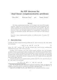
In Figure 1, we show that the PPA can also obtain very accurate solution for the
instance rand-500 reported in Table 3 without incurring substantial amount of additional
computing time. As can be seen from the figure, the time taken only grows almost linearly
when the required accuracy is geometrically reduced.
Table 3: Performance of the PPA on (3) with synthetic data (II).
problem m | n it/itsub/pcg pobj dobj R P /R D /R G /L loss
2 time
rand-500 112172 | 500 19| 42| 16.9 -3.13591727 2 -3.13589617 2 4.2-7| 9.5-7| 3.4-6| 1.7-2 82.6
rand-1000 441294 | 1000 20| 46| 24.0 -9.74364421 2 -9.74359627 2 8.6-7| 3.9-7| 2.5-6| 2.0-2 765.4
rand-1500 979620 | 1500 23| 56| 21.7 -1.91034252 3 -1.91033197 3 7.5-7| 4.7-7| 2.8-6| 1.8-2 2654.8
rand-2000 1719589 | 2000 22| 52| 20.9 -3.00395927 3 -3.00395142 3 9.8-7| 3.3-7| 1.3-6| 1.5-2 5353.4
130
120
110
time (seconds)
100
90
80
70
60
50
10 −4
10 −5
10 −6 10 −7
accuracy
10 −8
10 −9
Figure 1: Accuracy versus time for the random instance rand-500 reported in Table 3.
In Table 4, we compare the performance of our PPA and the ANS method on the
first three instances reported in Table 3. For the PPA, Tol in (31) is set to 3 × 10 −6 , 3 ×
10 −7 and 3 × 10 −8 ; for ANS, ɛ o is set to 10 −1 , 10 −2 and 10 −3 , and ɛ c is set to 10 −4 , so that
the gap (= |pobj − dobj|) can fall below 10 −1 , 10 −2 and 10 −3 , respectively. From Table
4, we can see that the PPA consistently outperforms the ANS method by a substantial
margin, which ranges from a factor of 5 to 26.
18

Table 4: Comparison of the PPA and the ANS method on (3) with
synthetic data (II).
problem m | n tolerance gap time
PPA (Tol) ANS (ɛ o , ɛ c ) PPA ANS PPA ANS
rand-500 112172 | 500 3 × 10 −6 (10 −1 , 10 −4 ) 5.58-3 9.79-2 75.7 518.3
3 × 10 −7 (10 −2 , 10 −4 ) 3.05-4 9.94-3 96.3 1233.2
3 × 10 −8 (10 −3 , 10 −4 ) 4.45-5 9.94-4 109.9 2712.3
rand-1000 441294 | 1000 3 × 10 −6 (10 −1 , 10 −4 ) 1.35-2 9.91-2 704.9 4499.8
3 × 10 −7 (10 −2 , 10 −4 ) 6.04-4 9.94-3 885.3 11715.4
3 × 10 −8 (10 −3 , 10 −4 ) 7.64-5 9.94-4 1006.6 26173.1
rand-1500 979620 | 1500 3 × 10 −6 (10 −1 , 10 −4 ) 2.23-2 9.94-2 2499.4 13601.7
3 × 10 −7 (10 −2 , 10 −4 ) 2.36-3 9.94-3 2964.2 32440.2
3 × 10 −8 (10 −3 , 10 −4 ) 2.51-4 9.94-4 3429.2 65773.7
In the second synthetic experiment, we consider the problem (4). We set ρ ij = 1/n 1.5
for all (i, j) ∉ Ω. We note that the parameters ρ ij are chosen empirically so as to give a
reasonably good value for ‖Σ − ̂Σ‖ F .
In Tables 5 and 6, we report the results in a similar format as those appeared in Table
3 and 4, respectively. Again, we may observe from the tables that the PPA outperformed
the ANS method by a substantial margin.
Table 5: Performance of the PPA on (4) with synthetic data (II).
problem m | n it/itsub/pcg pobj dobj R P /R D /R G time
rand-500 112172 | 500 25| 78| 18.2 -3.11255742 2 -3.11253082 2 6.5-8| 8.5-7| 4.3-6| 1.7-2 173.9
rand-1000 441294 | 1000 28| 100| 30.6 -9.70441465 2 -9.70433319 2 8.9-9| 4.7-7| 4.2-6| 2.0-2 2132.2
rand-1500 979620 | 1500 28| 89| 28.9 -1.90500086 3 -1.90497111 3 5.5-8| 9.4-7| 7.8-6| 1.8-2 5724.1
rand-2000 1719589 | 2000 30| 94| 26.5 -2.99725089 3 -2.99723060 3 2.1-8| 6.1-7| 3.4-6| 1.5-2 12217.7
Table 6: Comparison of the PPA and the ANS method on (4) with
synthetic data (II).
problem m | n tolerance gap time
PPA (Tol) ANS (ɛ o , ɛ c ) PPA ANS PPA ANS
rand-500 112172 | 500 3 × 10 −6 (10 −1 , 10 −4 ) 6.20-3 9.90-2 163.0 510.3
19

Table 6: Comparison of the PPA and the ANS method on (4) with
synthetic data (II).
problem m | n tolerance gap time
PPA (Tol) ANS (ɛ o , ɛ c ) PPA ANS PPA ANS
3 × 10 −7 (10 −2 , 10 −4 ) 4.94-4 9.94-3 196.1 1236.9
3 × 10 −8 (10 −3 , 10 −4 ) 9.24-5 9.94-4 218.1 2747.0
rand-1000 441294 | 1000 3 × 10 −6 (10 −1 , 10 −4 ) 4.45-2 9.88-2 1839.7 4460.8
3 × 10 −7 (10 −2 , 10 −4 ) 3.49-3 9.94-3 2278.7 11562.8
3 × 10 −8 (10 −3 , 10 −4 ) 2.75-4 9.94-4 2716.8 26278.6
rand-1500 979620 | 1500 3 × 10 −6 (10 −1 , 10 −4 ) 8.86-2 9.90-2 5254.1 13830.3
3 × 10 −7 (10 −2 , 10 −4 ) 3.36-3 9.94-3 6663.0 34208.0
3 × 10 −8 (10 −3 , 10 −4 ) 3.80-4 9.94-4 7605.1 73997.1
6.3 Real data experiments
In this part, we compare the PPA and the ANS method on two gene expression data sets.
Since [2] had already considered these data sets, we can refer to [2] for the choice of the
parameters ρ ij .
6.3.1 Rosetta Inpharmatics Compendium
We applied our PPA and the ANS method to the Rosetta Inpharmatics Compendium of
gene expression profiles described by Hughes et al. [9]. The data set contains 253 samples
with n = 6136 variables. We aim to estimate the sparse covariance matrix of a Gaussian
graphical model whose conditional independence is unknown. Naturally, we formulate it
as the problem (4), with Ω = ∅. As for the parameters, we set ρ ij = 0.0313 as in [2].
As our PPA can only handle problems with matrix dimensions up to about 3000, we
only test on a subset of the data. We create 3 subsets by taking 500, 1000, and 2000
variables with the highest variances, respectively. Note that as the variances vary widely,
we normalized the sample covariance matrices to have unit variances on the diagonal.
In the experiments, we set Tol = 10 −6 for the PPA, and (ɛ o , ɛ c ) = (10 −2 , 10 −6 ) for the
ANS method.
The performances of the PPA and ANS methods for the Rosetta Inpharmatics Compendium
of gene expression profiles are presented in Table 7. From Table 7, we can see
that although both methods can solve the problem, the PPA is nearly two times faster
than the ANS method when n = 1500.
20

Table 7: Comparison of the PPA and ANS method on (4) with
Ω = ∅ for the Rosetta Inpharmatics Compendiuma data.
problem m | n tolerance primal objective value time
PPA (Tol) ANS (ɛ o ) PPA ANS PPA ANS
Rosetta | 500 10 −6 10 −3 -7.42643038 2 -7.42642052 2 112.7 127.6
Rosetta | 1000 10 −6 10 −3 -1.66546574 3 -1.66546478 3 679.7 881.6
Rosetta | 1500 10 −6 10 −3 -2.64937821 3 -2.64937721 3 1879.8 3424.7
6.3.2 Iconix Microarray data
Next we analyze the performances of the PPA and ANS methods on a subset of a 10000
gene microarray data set obtained from 160 drug treated rat livers; see Natsoulis et al.
[15] for details. In our first test problem, we take 200 variables with the highest variances
from the large set to form the sample covariance matrix S. The other two test problems
are created by considering 500 and 1000 variables with the highest variances in the large
data set. As in the last data set, we normalized the sample covariance matrices to have
unit variances on the diagonal.
As the conditional independence of the Gaussian graphical model is not known, we
set Ω = ∅ in the problem (4). We set ρ ij = 0.0853 as in [2].
The performance of the PPA and ANS methods for the Iconix microarray data is
presented in Table 8. From the table, we see that the PPA is about two times faster than
the ANS method when n = 1000.
Table 8: Comparison of the PPA and ANS method on (4) with
Ω = ∅ for the Iconix microarray data.
problem m | n tolerance primal objective value time
PPA (Tol) ANS (ɛ o ) PPA ANS PPA ANS
Iconix | 200 10 −6 10 −3 -6.13127764 0 -6.13036186 0 51.5 50.7
Iconix | 500 10 −6 10 −3 5.31683807 1 5.31688551 1 571.6 795.2
Iconix | 1000 10 −6 10 −3 1.78893456 2 1.78892330 2 3510.8 7847.3
7 Concluding remarks
We designed a primal PPA to solve log-det optimization problems. Rigorous convergence
results for the PPA are obtained from the classical results for a generic proximal
21

point algorithm. Extensive numerical experiments conducted on log-det problems arising
from sparse estimation of inverse covariance matrices in Gaussian graphical models using
synthetic data and real data demonstrated that our PPA is very efficient.
In contrast to the case for the linear SDPs, the log-det term used in this paper plays
a key role of a smoothing term such that the standard smooth Newton method can be
used to solve the inner problem. The key discovery of this paper is the connection of the
log-det smoothing term with the technique of using the squared smoothing function. It
opens up a new door to deal with nonsmooth equations and understand the smoothing
technique more deeply.
Acknowledgements
We thank Onureena Banerjee for providing us with part of the test data and helpful
suggestions and Zhaosong Lu for sharing with us his Matlab code and fruitful discussions.
References
[1] F. Alizadeh, J. P. A. Haeberly, and O. L. Overton, Complementarity and nondegeneracy
in semidefinite programming, Mathemtical Programming, 77 (1997), 111–128.
[2] O. Banerjee, L. El Ghaoui, A. d’Aspremont, Model selection through sparse maximum
likelihood estimation, Journal of Machine Learning Research, 9 (2008), 485–516.
[3] R. Bhatia, Matrix Analysis, Springer-Verlag, New York, 1997.
[4] J. F. Bonnans and A. Shapiro, Perturbation Analysis of Optimization Problems,
Springer, New York, 2000.
[5] S. Boyd, L. El Ghaoui, E. Feron, and V. Balakrishnan, Linear matrix inequalities
in system and control theory, vol. 15 of Studies in Applied Mathematics, SIAM,
Philadelphia, PA, 1994.
[6] Z. X. Chan and D. F. Sun, Constraint nondegeneracy, strong regularity and nonsigularity
in semidenite programming, SIAM Journal on optimization, 19 (2008),
370–396.
[7] J. Dahl, L. Vandenberghe, and V. Roychowdhury, Covariance selection for nonchordal
graphs via chordal embedding, Optimization Methods and Software, 23 (2008),
501–520.
[8] A. d’Aspremont, O. Banerjee, and L. El Ghaoui, First-order methods for sparse
covariance selection, SIAM Journal on Matrix Analysis and Applications, 30 (2008),
56–66.
22

[9] T. R. Hughes, M. J. Marton, A. R. Jones, C. J. Roberts, R. Stoughton, C. D.
Armour, H. A. Bennett, E. Coffey, H. Dai, Y. D. He, M. J. Kidd, A. M. King, M.
R. Meyer, D. Slade, P. Y. Lum, S. B. Stepaniants, D. D. Shoemaker, D. Gachotte,
K. Chakraburtty, J. Simon, M. Bard, and S. H. Friend, Functional discovery via a
compendium of expression profiles, Cell, 102(1) 2000, 109C-126.
[10] Z. Lu, Smooth optimization approach for sparse covariance selection, SIAM Journal
on Optimization, 19(4) (2009), 1807–1827.
[11] Z. Lu, Adaptive first-order methods for general sparse inverse covariance selection,
Manuscript, Department of Mathematics, Simon Fraser University, Canada, December
2008.
[12] F. Meng, D. F. Sun, and G. Zhao, Semismoothness of solutions to generalized equations
and the Moreau-Yosida regularization, Mathemtical Programming, 104 (2005),
561–581.
[13] G. J. Minty, On the monotonicity of the gradient of a convex function, Pacific Journal
of Mathematics, 14 (1964), 243–247.
[14] J. J. Moreau, Proximitá et dualitá dans un espace Hilbertien, Bulletin de la Société
Mathématique de France, 93 (1965), 273–299.
[15] Georges Natsoulis, Cecelia I Pearson, Jeremy Gollub, Barrett P Eynon, Joe Ferng,
Ramesh Nair, Radha Idury, May D Lee, Mark R Fielden, Richard J Brennan, Alan
H Roter and Kurt Jarnagin, The liver pharmacological and xenobiotic gene response
repertoire, Molecular Systems Biology, 175(4) (2008), 1–12.
[16] Yu. E. Nesterov, Smooth minimization of nonsmooth functions, Mathemtical Programming,
103 (2005), 127–152.
[17] R. T. Rockafellar, Convex Analysis, Princeton University Press, Princeton, 1970.
[18] R. T. Rockafellar, Monotone operators and the proximal point algorithm, SIAM Journal
on Control and Optimization, 14 (1976), 877–898.
[19] R. T. Rockafellar, Augmented Lagrangains and applications of the proximal point
algorithm in convex programming, Mathematics of Operation Research, 1 (1976),
97–116.
[20] D. F. Sun, J. Sun and L. W. Zhang, The rate of convergence of the augmented
Lagrangian method for nonlinear semidefinite programming, Mathematical Programming,
114 (2008) 349–391.
23

[21] K .C. Toh, Primal-dual path-following algorithms for determinant maximization problems
with linear matrix inequalities, Computational Optimization and Applications,
14 (1999), 309–330.
[22] R. H. Tütüncü, K. C. Toh, and M. J. Todd, Solving semidefinite-quadratic-linear
programs using SDPT3, Mathemtical Programming 95 (2003), 189–217.
[23] N. -K. Tsing, M. K. H. Fan, and E. I. Verriest, On analyticity of functions involving
eigenvalues, Linear Algebra and its Applications 207 (1994), 159–180.
[24] L. Vandenberghe, S. Boyd, and S. -P. Wu, Determinant maximization with linear
matrix inequality equalities, SIAM Journal on Matrix Analysis and Applications, 19
(1998), 499–533.
[25] W. B. Wu, M. Pourahmadi, Nonparameteric estimation of large covariance matrices
of longitudinal data, Biometrika, 90 (2003), pp. 831–844.
[26] F. Wong, C. K. Carter, and R. Kohn, Efficient estimation of covariance selection
models, Biometrika, 90 (2003), pp. 809–830.
[27] K. Yosida, Functional Analysis, Springer Verlag, Berlin, 1964.
[28] X. Y. Zhao, D. F. Sun, and K. C. Toh, A Newton-CG augmented Lagrangian method
for semidefinite programming, preprint, National University of Singapore, March
2008.
24