Vegetation Radiative Transfer Modelling (Nadine Gobron) - PEER

Radiative Transfer Modeling 

…. over vegetated surfaces 

Nadine Gobron 

Global Environmental Unit, TP 440 

Email: nadine.gobron@jrc.it 

1

Scientific Context 

• Earth observing satellites are a unique tool with which to 

objectively monitor terrestrial environments at the global scale. 

• Temporal changes in the biosphere can be monitored using advanced 

methods to interpret remote sensing data. 

• The aim of these methods is to provide measurable parameters representing 

the state of the terrestrial surfaces. 

• These remote sensing products constitute reliable indicators of the 

evolution of the living biosphere. 

• In practice, one does acquire the measurements from the satellite, and would 

like to know what is going on in the environment: 

This is the inverse problem: Knowing the value of the electromagnetic 

measurements gathered in space, how can we derive the properties of the 

environment that were responsible for the radiation to reach the sensor? 

2

Satellites have different “eyes” 

Swath 1150 km – Res. 300m to 1.2 km 

Swath 2800 km – Res. 1.5 km 

MERIS/ENVISAT 

Swath 2330 km – Res. 250m to 1.1 km 

MODIS/TERRA 

Swath 200 km – Res. 500m 

MOS/IRS P3 

79 km 

Credit: NASA/GSFC/LaRC/JPL MISR Team 

Swath 979 km – Res. 275 m to 1.0 km 

SeaWiFS/OrbView 

3

How is remote sensing exploited? 

• The signals detected by the sensors are immediately converted 

into digital numbers and transmitted to dedicated receiving 

stations, where these data are heavily processed. 

• The effective exploitation of remote sensing data to reliably 

generate useful, pertinent information hinges on the 

availability and performance of specific tools and techniques 

of data analysis and interpretation. 

• A variety of mathematical models can be used for this 

purpose; they are implemented as computer codes that read the 

data or intermediary products and ultimately lead to the 

generation of products and services usable in specific 

applications…. User is happy ! 

4

Model of radiation transfer 

• Since space borne instruments can only measure the properties 

of electromagnetic waves emitted or scattered by the Earth, 

scientists need first to understand where these waves originate 

from, how they interact with the environment, and how they 

propagate towards the sensor. 

• To this effect, they develop models of radiation transfer, 

assuming that everything is known about the sources of 

radiation and the environment, and calculate the properties of 

the radiation field as the sensor should measure them. This is 

the so-called direct problem. 

5

Radiative Transfer Modeling 

• In solar domain, radiation transfer models are tools to 

represent the scattering and absorption of radiation by 

scattering elements/centers. They should satisfy energy 

conservation. 

• Spectral properties are depending 

on the geophysical medium: 

atmosphere, ocean, soil, 

or vegetation 

• Monograph dealing with 

RT problems in geophysics 

(Chandrasekhar (1960), 

Van de Hulst (1957), 

Lenoble (1993), Hapke (1993), 

Liou (1980) etc…) mainly concentrate on mathematical 

issues related to solving equations. 

• Rather than discussing the solving of approximate equations 

applicable to realistic geophysical situations, we will 

concentrate on exact and light mathematical treatment of a 

simplified physical system… 

6

Outline 

• Radiative Transfer Equations 

• Radiative Transfer Modeling for vegetation 

canopy. 

• Inversion problem for the retrieval of land 

products with actual remote sensing data. 

7

Radiative Transfer Equations (1) 

• Exact and light mathematical treatment of a simplified 

physical system 

• The system under consideration will have the following 

properties: 

– A continuous scattering-absorbing medium, infinite in lateral extent, bounded 

by two parallel planes, i.e. a plane-parallel medium. 

– Radiation can be scattered in only two directions, upward and downward. 

z=0 

z 

z+Δz 

z=z h 

Pinty, B. and M. M. Verstraete (1998) `Introduction to Radiation Transfer Modeling in Geophysical Media’, in From Urban 

Air Pollution to Extra-Solar Planets, ERCA Volume 3 Edited by C. Boutron, EDP Sciences, Les Ulis, France, 67-87. 

8

• The system under consideration will have the following 

properties: 

– Radiation or “ensemble of photons” is emitted by sources outside the 

medium only. 

– The amount of mean monochromatic radiant energy traveling upward 

and downward that crosses a unit area per unit time is an intensity 

noted I [Wm -2 sr -1 ]. 

Radiative Transfer Equations (1) 

z=0 

I (z) 

I (z+Δz) 

I (z) 

I (z+Δz) 

z 

z+Δz 

z=z h 



9

Basic Processes (1) 

Scattering 

“A physical process by which an ensemble of particles 

immerged into an electromagnetic radiation field remove 

energy from the incident waves to re-irradiate this energy into 

other directions” 

Absorption 



energy from the incident waves to convert this energy in a 

different form” 

Extinction 



energy from the incident waves to attenuate the energy of this 

incident wave” 

10

Basic Processes (2) 

•The upward and downward intensities change along the vertical coordinate z 

in the medium according to the volumetric (individual cross-sections times the 

number per unit volume) coefficients of absorption, K (in m -1 ) and scattering S 

(in m -1 ) 

•Thus 1/S (1/K) have dimensions of length and may be interpreted as the 

absorption (scattering) mean free paths, i.e. the average distance between 

absorption (scattering) events. 

z=0 

I (z) 

I (z+Δz) 

I (z) 

I (z+Δz) 

z 

z+Δz 

z=z h 

11

I (z) 

I (z+Δz) 

Conservation of radiant energy 

for I in a slab Δz 

I (z) 

I (z+Δz) 

z=0 

z 

z+Δz 

z=z h 

P is the probability 

that a photon 

directed upward is 

scattered downward 

I 

↓ 

(z) 

+ 

SΔzP 

↑↓ 

I 

↑ 

(z 

+ 

Δz) 

= 

P is the probability 

that a photon 

directed downward 

is scattered upward 

↓ 

↓↑ 

KΔ zI (z) + SΔzP 

I (z) + I (z + 

↓ 

↓ 

Δz) 

coefficients of absorption, K (in m -1 ) and scattering S (in m -1 ) 

12

Conservation of radiant energy for I in a slab Δz 

z=0 

I (z) 

I (z+Δz) 

I (z) 

I (z+Δz) 

z 

z+Δz 

z=z h 

I 

↑ 

(z 

+ 

Δz) 

+ 

SΔzP 

↓↑ 

I 

↓ 

(z) 

= 

KΔzI 

↑ 

(z 

↑↓ 

+ Δz) 

+ SΔzP 

I (z + Δz) 

↑ 

+ 

I 

↑ 

(z) 


13

Conservation of radiant energy in a slab Δz 

We obtain the two-stream equations 

∂I 

↓ 

∂z 

(z) 

= −KI 

↓ 

(z) 

− 

SP 

↓↑ 

I 

↓ 

(z) 

+ 

SP 

↑↓ 

I 

↑ 

(z) 

∂I 

↑ 

∂z 

(z) 

= + KI 

↑ 

(z) 

+ 

SP 

↑↓ 

I 

↑ 

(z) 

− 

SP 

↓↑ 

I 

↓ 

(z) 




14

Asymmetry factor for scattering processes 

•We have for isotropic medium: 

P 

↑↓ = P ↓↑ 

•The asymmetry factor g is a single number, defined as the 

mean cosine of the scattering angle (-1 or +1 in our case): 

↓↓ 

↓↑ 

g 

= ( + 1)P + ( −1) 

P 

•Typically: g = +1 for strict downward scattering, 

g=-1 for strict upward scattering and, 

g=0 for isotropic scattering. 

•For the above set of equations, we have: 

P 

↑↓ 

P 

↓↓ = P ↑↑ 

↑↑ ↓↑ ↓↓ 

+ P = P + P = 1 

P 

↑↓ = P 

↓↑ = (1 − g) / 2 

P ↑↑ = P 

↓↓ = (1 + g) / 2 

15

Single scattering albedo 

•Normalization of the radiation transport equations by the 

extinction factor E=S+K gives : 

↓ 

1 ∂I 

(z) K ↓ S ↓↑ ↓ S ↑↓ ↑ 

= − I (z) − P I (z) + P I (z) 

E ∂z 

E E E 

which can be rewritten as: 

1 ↓ 

↓ 

↑ 

E 

↓ 

∂I 

(z) 

∂z 

= −I 

(z) + 

(1 + g) 

ω 

2 

(z) + 

(1 − g) 

ω 

2 

↑ 

1 ∂I 

(z) ↑ (1 + g) ↑ (1 − g) ↓ 

= + I (z) − ω I (z) − ω I (z) 

E ∂z 

2 

2 

where is called the single scattering albedo 

S S 

ω = = 

S + K E 

expressing the probability for the photons to be scattered. 



I 

I 

(z) 

16

Single scattering albedo 

↓ 

∂I 

(z) 

E ∂z 

↑ 

∂I 

(z) 

E ∂z 

1 ↓ 

↓ 

↑ 

= −I 

= + I 

(1 + g) 

(z) + ω I 

2 

(1 + g) 

(z) − ω I 

2 

(1 − g) 

(z) + ω I 

2 

(1 − g) 

(z) − ω I 

2 

1 ↑ 

↑ 

↓ 

(z) 

(z) 

ω = 

S 

S + K 

= 

S 

E 

• Single scattering albedo ω =0 for total absorption (no 

scattering) 

• Single scattering albedo ω =1 for total or conservative 

scattering (no absorption) 



17

Optical thickness 

• The variable physical depth can be multiplied by the 

optical factor S+K=E to transform into an optical thickness 

↓ 

∂I 

(z) 

∂τ 

τ 

= −I 

↓ 

z 

∂z 

= ∫ (S + K) ∂z 

0 

(1 + g) 

(z) + ω 

2 

I 

↓ 

(1 − g) 

(z) + ω 

2 

I 

↑ 

(z) 

∂τ 

(1) 

↑ 

∂I 

(z) 

∂τ 

= + I 

↑ 

(z) 

− 

ω 

(1 + g) 

2 

I 

↑ 

(z) 

− 

ω 

(1 − g) 

2 

I 

↓ 

(z) 

(2) 

These last equations are typical two-stream equations 

for the system. 



18

Two-stream equations 

• In a more compact form [with (1) - (2) and (1)+(2)]: 

↓ ↑ 

∂( I − I ) 

↓ ↑ 

= −(1 

− ω)(I 

+ I ) 

∂τ 

↓ ↑ 

∂( I + I ) 

↓ ↑ 

= −(1 

− ωg)(I 

− I ) 

∂τ 

Key variables to represent the radiative transfer processes are: 

• ω : the single scattering albedo 

• g : the asymmetry factor of the phase function 

• τ : the optical thickness of the medium 



19

Extension to N Flux (1) 

• These equations can be extended to N flux to obtain N 

coupled differential equations including N+1 terms on 

the right side. 

•The first term represents the extinction and the N 

remaining terms represent all the possible ways in which 

radiation is scattering into one direction Ω from all other 

directions Ω’. 

•In the limit when N goes to infinity, sums become 

integrals and the set of equations collapses into a single 

integro-differential equation: 

∂I 

( z, 

Ω) 

− μ 

∂τ 

+ ~ σ ~ 

e 

( z, 

Ω) 

I( 

z, 

Ω) 

= σ s 

( z, 

Ω' 

→ Ω) 

I( 

z, 

Ω') 

dΩ' 



∫ 

4Π 

20

Extension to N Flux (2) 

In the limit when N goes to infinity, sums become integrals and 

the set of equations collapses into a single integro-differential 

equation: 

∂I 

( z, 

Ω) 

− μ 

∂τ 

+ ~ σ ~ 

e 

( z, 

Ω) 

I( 

z, 

Ω) 

= σ s 

( z, 

Ω' 

→ Ω) 

I( 

z, 

Ω') 

dΩ' 

I (z, Ω ) represents the intensity (W m -2 sr -1 ) at point z in the 

exiting direction Ω, 

σ e (m -1 ) and σ s (m -1 sr -1 ) are the extinction and differential 

scattering coefficients, respectively, taken at the same point z 

along the direction Ω. 

∫ 

4Π 



21

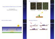
Vertical radiative coupling between 

geophysical media 

Atmosphere 

Vegetation 

Soil 

Upper limit (1) 

RTE 

Lower Limit (1) 


RTE 



RTE 


Z A 

Z V 

Z S 

In each medium, the transfer of radiation may be represented 

by the following approximate equation: 

∂ 

[ −μ 

+ ~ σ ~ 

e 

( z, 

Ω, 

ΩO)] 

I( 

z, 

Ω) 

= ∫σ 

s 

( z, 

Ω' 

→ Ω) 

I( 

z, 

Ω') 

dΩ' 

∂τ 

Extinction coefficient 

Differential 

4Π 

scattering coefficient 



22

Atmosphere 


Soil 



•Non oriented small scatterers 

•Infinite number of scatterers 

•Low density turbid medium 

•Oriented finite-size scatterers 

•Finite number of scatterers 

•Dense discrete medium 

•Oriented small-size scatterers 

•Infinite number of clustered scatterers 

•Compact semi-infinite medium 



23



The description of the interaction of a radiation field with a 

layered geophysical medium implies the solution of 

radiation transfer equations and the specification of 

appropriate boundary conditions 

I 

↓ 

Atmosphere 

Soil 

( z ta 

, Ω) 

= I0δ 

( Ω − Ω 

o 

) 

I ↑ ( z , Ω) 

= 

∞ 

0 

I 

↑ 

( , Ω) 

↑ 

1 

' ↓ 

' ' 

I ( z 

ba 

, Ω ) = ( , Ω , Ω ) ( 

, 

Ω ) | | Ω 

Π 

∫ γ 

v 

z 

ba 

I z 

ba 

μ d 

2 Π 

↓ 

↓ 

− τ 

a ↓ 

I ( z 

tv 

, Ω ) = I ( z 

ta , 

Ω ) exp[ ] + I 

d 

( z 

ba 

, Ω ) 

| μ 

0 

| 


↑ 

1 

' ↓ 

' ' ' 

I ( z 

bv 

, Ω ) = ( , Ω , Ω ) ( 

, 

Ω ) | | Ω 

Π 

∫ γ 

s 

z 

bv 

I z 

bv 

μ d 

2 Π 



z a 

' 

Z a 

Z V 

Z S 

24

Outline 



canopy. 



25

Representation of vegetation canopy 

‘Oriented’ scatterers elements in a finite volume 

turbid medium 

» Leaves are point-like scatterers 

discrete medium 

» Leaves are finited-size scatterers 

26

Discrete canopy: 1D representation 

Df 

H 

Geometrical Parameters in 1D representation: 

Height of canopy, Size of a single leaf & Leaves 

orientation (leaf angle distribution) 

Gobron, N et. al. (1997) ‘A semi-discrete model for the scattering of light by vegetation’, Journal of Geophysical Research, 

102, 9431-9446. 

27

Vegetation ‘Optical Depth’ 

• Leaf Area Index (LAI) is a quantitative 

measure of the amount of live green leaf 

material present in the canopy per unit ground 

surface. 

• It is defined as the total one-sided area of all 

leaves in the canopy within a defined region. 

N N 

LAI = ∑ λ ∑ i = niai 

i= 

1 i= 

1 

N = # of layers 

a i = leaf surface 

n i = # leaves /m2 


102, 9431-9446. 

28

Vegetation ‘Optical Depth’ 

• Leaf Area Index (LAI) is a quantitative 

measure of the amount of live green leaf 

material present in the canopy per unit ground 

surface. 

• It is defined as the total one-sided area of all 

leaves in the canopy within a defined region. 

H : Height of canopy [m] 

LAI = H.Δ 

Δ : Leaf Area Density [m 2 /m 3 ] 


102, 9431-9446. 

29

Geometrical System 

Ωo 

θ 

Ω 

φ 

North 

φ ο 

H 

θ ο 

z 


102, 9431-9446. 

30

~ Extinction coefficient σ ( z, 

Ω, 

ΩO) 

e 

∂ 

[ −μ 

+ ~ σ ~ 

e 

( z, 

Ω, 

ΩO)] 

I( 

z, 

Ω) 

= ∫σ 

s 

( z, 

Ω' 

→ Ω) 

I( 

z, 

Ω') 

dΩ' 

∂τ 

We assume that the canopy consists of plane leaves with a leaf area 

density λ(z) defined to be the total one-sided leaf area per unit volume 

at depth z. 

The probability that a leaf has a normal Ω 

directed away from the top surface, in a unit 

solid angle about 

Ω l 

is given by the leaf-normal distribution function 

which is normalized as 

1 

2π 

∫ 

2π 

dφ 

l 

1 

∫ 

0 

dμ 

l 

g 

l 

4Π 

l 

( z, 

Ω 

⎜ 

⎛ 

⎝ 

l 

θ 

) 

l 

g 

, ϕ 

l 

= 

l 

⎟ 

⎞ 

⎠ 

( z, 

Ωl) 

1 

Ω L 

plate model 31

Extinction coefficient 

We now consider photons at a depth z traveling in direction Ω. 

The extinction coefficient is then the probability, per unit path length, 

that the photon hits a leaf, i.e., the probability that a photon while 

traveling a distance ds along Ω is intercepted by a leaf divided by the 

distance ds. 

e 

( z, ) G( z, 

) ( z) 

σ Ω = Ω λ 

Where the geometry factor G is the fraction of the total leaf area (per 

unit volume of the canopy) that is perpendicular to Ω 

1 

G ( z, 

) = ( Ω ) | Ω • Ω | 

l l 

2π 

2π 

Ω ∫ g 

d 

l 

Ω 

l 

Ross J. (1981) ‘The Radiation Regime and Architecture of Plant Stands’, The Hague-Boston-London: Dr. W.Junk 

Publishers, 391 pp. 

32

Leaf Orientations 

Vegetation foliage features characteristic leaf-normal distributions, 

g(Ω L ) with preferred: 

• azimuthal orientations, g(φ L ) 

• zenithal orientations, g(θ L ): 

‣ erectophile (grass) (90 o ) 

‣ planophile (water cress) (0 o ) 

‣ plagiophile (45 o ) 

‣ extremophile (0 o and 90 o ) 

‣ uniform/spherical (all) 

• time varying orientations: 

‣ heliotropism (sunflower) 

‣ para-heliotropism 

Ross J. (1981) ‘The Radiation Regime and Architecture of Plant Stands’, The Hague-Boston-London: Dr. W.Junk 

Publishers, 391 pp. 

33

Scattering properties of leaves 

• Once the radiation is intercepted by the vegetation elements, it 

is scattered in directions determined by the leaf orientations and 

the leaf phase function 

Ω 

• Leaf reflection and transmission 

depend primarily on wavelength, 

plant species, growth condition, 

age and position in canopy. 

• Directionality of leaf scattering 

depends on the leaf surface 

roughness, and the percentage 

of diffusely scattered photons 

from leaf interior. 

Ω 

Ω L 

plate model 

‣ Plate models often assume Bi-Lambertian scattering properties: 

- radiation is scattered according to cosine law: | Ω L · Ω | 

- magnitude depends on leaf reflection and transmission values 

34

Leaf scattering properties 

• Leaf scattering function for classical plate scattering 

model 

f ( Ω 

' 

→ 

Ω, 

Ω 

l 

) 

= 

r 

l 

| 

Ω • Ω | 

l 

/ 

π 

if ( Ω • Ω )( Ω 

l 

' 

• Ω ) 

l 

< 

0 

f ( Ω 

' 

→ 

Ω, 

Ω 

l 

) 

= 

t 

l 

| 

Ω • Ω | 

l 

/ 

π 

if ( Ω • Ω )( Ω 

l 

' 

• Ω ) 

l 

> 

0 

Where r l and t l are the fraction of intercepted energy 

which are reflected (transmitted) following a simple 

cosine distribution law around the normal to the 

leaves. 

35

Reflectance measurements of leaves 

Summer - Autumn - Winter 

60 

40 

20 

Chlorophyls 

Anthocyans 

Tannins 

0 

200 600 1000 1400 1800 2200 2600 

nm 

brown leaf red leaf green leaf 

Source: B. Hosgood 

36

Canopy scattering phase function 

• Leaf properties are assumed to be the same throughout 

the canopy, we have 

1 

π 

1 

π 

Γ(z 

k 

Γ( 

Ω 

, Ω 

' 

' 

→ 

→ 

Ω) 

Ω) 

≡ 

≡ 

1 

2π 

1 ' 

Γ( 

Ω → Ω) 

π 

∫ 

2π 

g( Ω 

l 

) | Ω 

' 

• Ω | f ( Ω 

' 

→ 

Ω, 

Ω 

l 

)dΩ 

l 

g (Ω L ) is the probability function for the leaf normal distribution Ω L 

f is the leaf phase function (when integrated over all exit photons 

directions, yields single scattering albedo ω). 

Shultis, J. K. and Myneni, R. B. (1988) ‘Radiative transfer in vegetation canopies with an isotropic scattering’, Journal of 

quantitative spectroscopy and radiative transfer 39: 115-- 129. 

37 

Knyazihin et. al. (1992) ‘Interaction of Photons in a Canopy of Finite Dimensional Leaves’, Remote Sens. Envir., 39:61-74.

Specific Effects 

•The presence of finite size scatterers implies that the radiation 

interception process by the leaves will not follow a continuous 

scheme, and in particular that radiation will be allowed to 

travel unimpeded within the free space between the scatterers. 

•Since extinction occurs only at discrete locations, some of the 

radiation emerging from an arbitrary source, located inside or 

outside the canopy, any occasionally travel without any 

interaction in this canopy, depending on the shape and size of 

free space between these leaves. 

Verstraete, M. M et. al. (1990) 'A physical model of the bidirectional reflectance of vegetation canopies; Part 1: Theory', Journal of 

Geophysical Research, 95, 11,755-11,765. 

Gobron, N et. al. (1997) ‘A semi-discrete model for the scattering of light by vegetation’, Journal of Geophysical Research, 102, 38 

9431-9446.

•When the radiation is scattered 

back in the direction from which it 

originates, the probability of further 

interaction with the canopy is lower 

than in other scattering directions. 

•In case of RS measurements 

outside the canopy, this give rise to 

a relative increase in the value in 

the backscattering direction which 

is knows as the hot-spot 

phenomenon. 

Hot-spot Effects 




9431-9446.

Hot-spot Effects 

Extinction coefficient is modified adding hot-spot 

scale factor: 

σ e (z, Ω, Ω 0 ) = Λ(z) · G(Ω)· O(z, Ω, Ω 0 ) 

Ω 0 

Ω = Ω 0 

Ω 

Turbid canopy representation: 1-D 

-90 -45 0 45 90 

observation zenith angle [degree] 

illuminated leaf 




9431-9446. 

Bi-directional Reflectance Factor (λ= Red) 

0.08 

0.06 

0.04 

0.02 

0.00 

1-D’ 

1-D

Separation of Scattering Order 

ρ ( z0, 

Ω, 

Ω0) 

= ρ 0 (z0, 

Ω, 

Ω0) 

+ ρ 1 (z0, 

Ω, 

Ω0) 

+ ρ M (z0, 

Ω, 

Ω0) 

• Uncollided intensity 

• Single Collided intensity 

• Multiple scattering intensity 

Gobron, N et. al. (1997) ‘A semi-discrete model for the scattering of light by vegetation’, Journal of Geophysical 

Research, 102, 9431-9446. 

41

Uncollided intensity (1) 

Downward uncollided intensity at level z k 

Where 

I 

0 

↓ 

(z 

k 

, Ω 

0 

) = 

I 

s 

⎡ 

⎢1 

− λ 

⎣ 

0 

Is 

= I (z0, 

Ω0) 

δ( 

Ω − Ω0) 

G( Ω0) 

⎤ 

⎥ 

| μ | ⎦ 

0 

k 

is the incoming 

collimated beam at the top of canopy 

Probability that a light ray within this beam is transmitted 

downward in the same direction through the first k layers 


Research, 102, 9431-9446. 

42

I 

0 

↑ 

(H, Ω, 

Ω 

0 

) 

= 

1 

π 

γ 

s 

Uncollided intensity (2) 

The radiation scattered by the soil, which provides the lower 

radiative boundary condition of the canopy system, for 

uncollided radiation is given by: 

γ 

( H, Ω, 

Ω0) 

(H, Ω, 

Ω 

0 

) 

| 

μ 

0 

| 

I 

s 

⎡ 

⎢1 

− λ 

⎣ 

G( Ω0) 

⎤ 

⎥ 

| μ | ⎦ 

Where s 

denotes the bidirectional reflectance 

factor of the soil at the bottom of canopy. 

0 

K 

I 

K 

k 

∏ + 1 

1 

⎡ G( Ω ⎤ ⎡ 

↑ = 

⎢ − 

0) 

⎢ − 

' G( Ω 

0 (zk, 

Ω, 

Ω 

) 

0) 

γs(H, 

Ω, 

Ω0) 

| μ0 

| Is 

1 λ 

1 λK 

π 

| μ0 

| j= 

K μ 

⎣ 

⎥ 

⎦ 

⎣ 

⎤ 

⎥ 

⎦ 


Research, 102, 9431-9446. 

43

Uncollided BRF 

Applying last equation at the top of canopy and normalized by 

the intensity of the source of incoming direct solar radiation as 

well as by the reflectance of a Lambertian surface illuminated 

and observed under identical conditions (|μ 0 |/π) yields the 

contribution to the bidirectional reflectance factor due to this 

uncollided radiation, namely: 

⎡ G( Ω0) 

⎤ ⎡ ' G( Ω) 

⎤ 

ρ 0 (z0, 

Ω, 

Ω0) 

= γs(H, 

Ω, 

Ω0) 

⎢1 

− λ ⎥ 1 

K 

| 

0 

| 

⎢ − λ ⎥ 

⎣ μ ⎦ ⎣ μ ⎦ 

K 

K 


Research, 102, 9431-9446. 

44

Uncollided BRF in Principal Plan 

Solar Zenith Angle: 20 [deg] 

Solar Azimuth Angle: 0 [deg] 

Radius: 

0.05 [m] 

Leaf Area Index: 3.0 [ m2/m2] 

Height of the canopy: 2.0 [ m] 

Normal Distribution: Erectophile 

Leaf scattering law: Bi-Lambertian 

Leaf reflectance: 0.0546 

Leaf transmittance: 0.0149 

Soil scattering law: Lambertian 

Soil reflectance: 0.127 

http://rami-benchmark.jrc.it 

45

Uncollided BRF in Principal Plan 



Radius: 

0.05 [m] 





Leaf reflectance 0.4957 

Leaf transmittance 0.4409 

Soil scattering law Lambertian 

Soil reflectance 0.159 


46

Uncollided BRF in Cross Plan 



Radius: 

0.05 [m] 










47

First collided Intensity (1) 

The first collided intensity in downward direction Ω 

corresponds to the radiation scattered only once by leaves, 

but which has not interacted with the soil. 

•Downward source coming from the direct intensity, 

attenuated through the first k layers, and scattered by the 

leaves according to their optical properties in layer k: 

Q 

0 

↓ 

(z 

k 

, Ω, 

Ω 

•Downward intensity 

I 

1 

↓ 

(z 

k 

, Ω, 

Ω 

0 

) 

0 

) 

= 

1 

1 

Γ( 

Ω 

π 

0 

→ Ω)I 

s 

⎡ 

⎢1 

− 

⎣ 

G( Ω0) 

⎤ 

λ ⎥ 

| μ | ⎦ 

⎡ − 

⎣ 

k 

= ∑ 

0 

Q (zi, 

Ω, 

Ω0) 

λ 1 

↓ 

μ 

⎢ 

i= 

1 

λ 

| μ 


Research, 102, 9431-9446. 

0 

k 

G( Ω) 

⎤ 

| 

⎥ ⎦ 

48 

k−i

First collided Intensity (2) 

The first collided intensity in downward direction Ω 

corresponds to the radiation scattered only once by leaves, 

but which has not interacted with the soil. 

•Downward intensity 

I 

1 

↓ 

(z 

k 

, Ω, 

Ω 

0 

) 

•Upward intensity 

1 

⎡ − 

⎣ 

G( Ω) 

⎤ 

| 

⎥ ⎦ 

k 

= ∑ 

0 

Q (zi, 

Ω, 

Ω0) 

λ 1 

↓ 

μ 

⎢ 

i= 

1 

λ 

| μ 

k−i 

I 

1 

↑ 

(z 

k 

, Ω, 

Ω 

0 

) 

k+ 

1 

k+ 

1 

1 = ∑{ 

0 

Q (z × ∏ 

↓ i, 

Ω, 

Ω0) 

λ 

μ 

i= 

K 

j= 

i 

⎡ 

⎢1 

− 

⎣ 

λ 

' 

i 

G( Ω) 

⎤⎫ 

⎥⎬ 

| μ | ⎦⎭ 


Research, 102, 9431-9446. 

49

Single collided BRF 

The contribution to the bidirectional reflectance factor due to 

the first collided intensity is obtained after normalizing the 

upward intensity I 1 

( z 

by the incoming 

0, 

Ω, 

Ω ) 

↑ 0 

directional source of radiation at the top of canopy: 

ρ ( z 

1 

0 

, Ω, 

Ω 

0 

) 

= 

Γ 

( Ω → Ω ) 

μ | μ | 

0 

0 

i 

1 

⎡ G( 

Ω ⎤ 

0) 

⎡ ' G( 

Ω 

∑λ⎢1 

− λ ⎥ ⎢1 

− λK 

i= K | μ0 

| 

μ 

⎣ 

⎦ 

⎣ 

) ⎤ 

⎥ ⎦ 

i 


Research, 102, 9431-9446. 

50

Single Collided BRF in Principal Plan 



Radius: 

0.05 [m] 










51

Single Collided BRF in Cross Plan 



Radius: 

0.05 [m] 










52

Ω•∇I λ 

(x,Ω)+G(x,Ω)u L 

(x)I λ 

(x,Ω)= u L(x) 

π 

Multiple Scattering 

Multiple scattering intensities are computed solving 

RT equations using various numerical tools, like: 

• Discrete Ordinate Methods 

• δ-Eddington method 

• Adding-doubling 

• Two-streams 

∫ 

4π 

Γ λ 

(x,Ω→ Ω ′)I λ 

(x, Ω ′)d Ω ′ 

53

Multiple Scattering 


54

Outline 



canopy. 



55

Association of physical 

measurements, models & models 

representing the biosphere 

The process of fitting data, as seen by Subramanian Raman in Science with a Smile. 

56





57





58

Model Inversion 

• In general, the system of equations cannot be solved: 

– If K< M, the system is still under-determined 

– If K= M, measurements errors may prevent the 

identification of the exact solution 

– If K> M, the system is over-determined 

K depends on space observation strategy 

M depends on the RT model 

59

Space Observation Strategies 

• Mono-directional multi-spectral scanning 

sensor on a Sun-synchronous orbit 

single view of the same target during a 

given day (given Sun zenith angle) 

• Spinning sensor on a geostationary orbit 

multiple views of the same target during 

a given day (various Sun zenith angles) 

• Multi-directional multi-spectral sensor on 

a Sun-synchronous orbit 

60


Source: http://seawifs.gsfc.nasa.gov/SEAWIFS/SEASTAR/ 

61


• Mono-directional multi-spectral scanning 

sensor on a Sun-synchronous orbit 

single view of the same target during a 

given day (given Sun zenith angle) 

• Spinning sensor on a geostationary orbit 

multiple views of the same target during 

a given day (various Sun zenith angles) 

62

Overview of MISR 

Ref: http://www-misr.jpl.nasa.gov/mission/minst.html 

63

Spectral Sensor Properties 

SeaWiFS 

MISR 

MODIS 

MERIS 

64

Bidirectional Reflectance Factor 

at Top Of Canopy : Nadir View 

SeaWiFS 

MISR 

MODIS 

MERIS 

Semi-discret Model 

65


at Top Of Canopy : Nadir View 

SeaWiFS 

MISR 

MODIS 

MERIS 


66


at Top Of Canopy 

lai =8. 

lai=4. 

lai=2. 

lai=1. 

lai=5. 

lai=3. 

lai=1.5 

lai=0.5 

SeaWiFS 

MISR 

MODIS 

MERIS 


67

Bidirectional Reflectance Factor Top Of 

Atmosphere: Aerosols Optical Depth 

Visibility : 151.58 38.33 : 20.22 7.74 5.11 km 

SeaWiFS 

MISR 

MODIS 

MERIS 

6S Model 

Vermote et al. 1997, IEEE 

68

Fraction of Absorbed Photosynthetically 

Active Radiation (FAPAR) 

I ⇓ 

TOC 

I ⇑ 

TOC 

canopy 

I ⇑ 

S 

I ⇓ 

S 

soil 

FAPAR = [(I ⇓ 

TOC 

+I ⇑S )–(I ⇑ 

TOC 

+I ⇓S )] / I ⇓ 

TOC 

Monitoring this bio-geophysical variable in time provides important 

information on the productivity of the vegetation and permits us to estimate, 

for example, the effectiveness of plants to assimilate atmospheric carbon 

dioxide. 

69

Conceptual approach: 

Design of FAPAR algorithm 

Measurement in the blue spectral domain (which is more 

sensitive to atmospheric optical thickness) is used to 

decontaminate the measurements in the red and near-infrared 

bands, respectively. 

A parametric model is used to remove angular effects. 

The two rectified values in red and near-infrared bands are 

then combined together to derive the FAPAR value. 

Technical approach: 

A large set of instrument like data (TOA) are simulated with 

radiative transfer model in vegetation and atmosphere. 

Optimization of coefficients is achieved to derive three 

polynomials formulae. 

70

Scheme for the algorithm optimization 

~ 

Radiation Transfer Models 

BRF TOA BRF TOC 

Rectified Red 

FAPAR 

Angular/Atmospheric effects 

ρ( 

λ ) = 

i 

TOA 

ρ ( Ω 

F( 

Ω , Ω , k 

~ 

0 

v 

0 

~ 

, Ωv, 

λi 

) 

HG 

, Ω , ρ 

λi 

λi 

λic 

) 

Rectified NIR 

ρ 

Rred 

= g1[ 

ρ( 

λblu), 

ρ( 

λred)] 

ρ 

Rnir 

= g2[ 

ρ( 

λblu), 

ρ( 

λnir)] 

i 

~ 

g [ ρ ( λ ), ρ( 

λ )] → 

~ ρ 

blu 

~ 

i 

~ 

TOC 

λ 

i 

~ 

~ 

~ 

g [ ρ( 

λ ), ρ( 

λ )] = P( 

λ , λ ) / Q( 

λ , λ ) 

n 

i 

P( 

λ , λ ) = l 

i 

Q( 

λ , λ ) = l 

i 

j 

n1 

+ l 

n5 

n6 

+ l 

FAPAR = g 

j 

j 

n10 

0 

= 

( l 

04 

i 

~ 

( ρ( 

λ ) + l 

~ 

~ 

~ 

( ρ 

i 

~ 

( ρ( 

λ ) + l 

j 

~ 

, ρ 

n2 

n7 

ρ( 

λ ) ρ( 

λ ) + l 

01 Rnir 

2 

Rred 

) 

) 

) 

) 

2 

ρ( 

λ ) ρ( 

λ ) 

i 

i 

Rred 

i 

l ρ 

− ρ 

Rnir 

j 

j 

i 

2 

− l 

+ 

j 

+ l 

+ l 

ρ 

n3 

n8 

n11 

~ 

( ρ( 

λ ) + l 

~ 

( ρ( 

λ ) + l 

− l 

02 Rred 03 

2 

( l05 

− ρ 

Rnir 

) 

j 

j 

+ l 

Optimization 

Procedure 

n4 

n9 

g0( 

ρ 

Rred 

, ρ 

Rnir 

) → FAPAR 

06 

) 

) 

2 

2 

N. Gobron, et al. (2000) ‘Advanced Vegetation Indices Optimized for Up-Coming Sensors: Design, Performance and Applications’, 71 

IEEE Transactions on Geoscience and Remote Sensing, 38, 2489-2505.

RT model driven improvement for FAPAR 

Optimization Procedure 



RT model driven improvement for FAPAR 



JRC-FAPAR Algorithm 

Satellite Data 

BRF TOA View angles Sun angles 

Angular/Atmospheric `Rectification' 

Rectified Red Rectified NIR 

~ 

~ 

ρ( 

λ ) = 

i 

~ 

TOA 

ρ ( Ω 

F ( Ω , Ω , k 

0 

, Ωv, 

λi 

) 

HG 

, Ω , ρ 

ρ 

Rred 

= g1[ 

ρ( 

λblu 

), ρ( 

λred 

)] ρ 

Rnir 

= g 

2[ 

ρ( 

λblu 

), ρ( 

λnir 

)] 

v 

0 

λi 

λi 

λic 

) 

~ 

~ 

L2 products 

Fapar 

FAPAR 

= g0( 

ρ 

Rred 

, ρ 

Rnir 

) 



JRC-FAPAR products 

 

Equivalent physically-based algorithm are developed for 

SeaWiFS, MERIS, GLI, MODIS and MISR/Terra. 

 

A processing chain has been designed to deliver time series of 

geophysical products from SeaWiFS at a global scale from 

October 1997 onwards. 

 

Time-composite algorithm selects the “most representative 

day” in the 10-day and monthly period such that the FAPAR 

for this day is closest to the averaged value. 

The assumptions in RT models impacts on the illumination 

angle at about 50° limit. 

The instantaneous accuracy of FAPAR is about ±0.1 

75

The time composite algorithm 

1) Compute the temporal average and corresponding deviation of 

product , e.g. FAPAR, over the N-day period: 

T 

S 

= 

S 

T 

1 

∑ T 

S t) 

t= 

1 

T 

1 

( Δ 

T 

= | S( 

t) 

− S | 

S 

T 

∑ 

t= 

1 

is the number of valid days during the N-day period 

2) Select the “most representative day” in the N-days time 

series such that it corresponds to the value 

which minimizes | S( 

t) 

− S | 

NB: the procedure is applied twice sequentially to reject values outside the range 

S ± Δ 

T S 

Pinty, B., N. Gobron, F. Mélin & M. M. Verstraete (2002) ‘A Time Composite Algorithm Theoretical 76 

Basis Document’, Institute for Environment and Sustainability, EUR Report No. 20150 EN, 8 pp.

08/01 08/02 08/03 08/04 08/05 

08/06 08/07 08/08 08/09 08/10 

Daily to temporal composite 

08/1-10 08/1-31 

77

• JRC Products with SeaWiFS data (0.5°x0.5°, 

0.25°x0.25°,10 km x 10 km, 10-day & monthly) 

[1997/10-2005/06] 

(Gobron et al. 1999, 2001) 

http://fapar.jrc.it/ 

at Global Scale 

• ESA Products with MERIS data [2002-end 

of mission] (Gobron et al. 1999) 

http://envisat.esa.int/ 

78

Validation protocol 

• The performance for detecting various events 

(verisimilitude) is assessed against the time-series of 

well documented land surface features. 

• The comparison against ground-based estimates can 

be performed recognizing the following: 

– Categorization of land validation site in their 

respective radiative transfer regime (not shown 

here) 

– Series of approximation to derive FAPAR from 

ground-based measurement sets. 

79

Fire event 

(Pearsoll Peak, CA) 

FAPAR September 2002 

Long Time series of 10-day 

Active Fire Detection 2002 

The FAPAR values suddenly decline after the 2002 summer fire events and keep low values, by 

comparison to those obtained for the period 1998-2001, until the end of 2003. 

The 2003 FAPAR estimations suggest that the vegetation has not recovered from the 2002 fire 

stress. 

Gobron N., et. al. (2006) ‘Evaluation of FAPAR Products for Different Canopy Radiation Transfer 

Regimes: Methodology and Results using JRC Products Derived from SeaWiFS and Ground-based 

Estimations', JGR, DOI 10.1029/2005JD006511 

80

Rice 

(Pavia, IT) 

FAPAR July 2003 

Long Time series of 10-day 

The FAPAR values are stable over all years. 

The 2003 FAPAR estimations suggest that the growth period was in advance comparing to a normal 

year. 

Gobron N., et. al. (2006) ‘Evaluation of FAPAR Products for Different Canopy Radiation Transfer 

Regimes: Methodology and Results using JRC Products Derived from SeaWiFS and Ground-based 


81

0.5 

Ground-based Estimations 

• Three issues and caveats among others: 

- Date and time of acquisition 

SRF1: 09 July 2004 

Fapar 

0.45 

0.4 

0.35 

±0.1 

0.3 

+2 hours 

0.25 

0.2 

Source: M. Meroni (DISAFRI-Unitus) 

8.00 9.00 10.00 11.00 12.00 13.00 14.00 15.00 16.00 17.00 

82 

Time of day




- Spatial resolution: in-situ measurements at very high 

resolution (1 m) to be extrapolated at the medium 

resolution pixel (number and spatial distribution of the 

samples, impact of horizontal fluxes) 

FAPAR Measurements 

Widlowski J.-L., et. al. (2006) ‘Horizontal radiation transport in 3-D 

forest canopies at multiple spatial resolutions: Simulated impact on 

canopy absorption’, RSE 

83




- Spatial resolution: in-situ measurements at very high 

resolution (1 m) to be extrapolated at the medium 

resolution pixel (number and spatial distribution of the 

samples, impact of horizontal fluxes) 

- Approximation of FAPAR by the intercepted 

radiation (impact of woody elements), i.e. 

FAPAR (μ0) ≈ FIPAR (μ0) = 1-T(μ0) 

See … Gobron N., et. al. (2006) ‘Evaluation of FAPAR Products for 

Different Canopy Radiation Transfer Regimes: Methodology and 

Results using JRC Products Derived from SeaWiFS and Groundbased 


84

http://fapar.jrc.it/ 

85

http://rami-benchmark.jrc.it/ 

86

Vegetation Radiative Transfer Modelling (Nadine Gobron) - PEER

You also want an ePaper? Increase the reach of your titles

Delete template?

Save as template?