Unsteady aerodynamics of wings with an oscillating flap ... - Pegasus
Unsteady aerodynamics of wings with an oscillating flap ... - Pegasus
Unsteady aerodynamics of wings with an oscillating flap ... - Pegasus

Create successful ePaper yourself
Turn your PDF publications into a flip-book with our unique Google optimized e-Paper software.
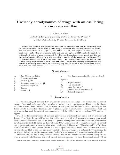
<strong>Unsteady</strong> <strong>aerodynamics</strong> <strong>of</strong> <strong>wings</strong> <strong>with</strong> <strong>an</strong> <strong>oscillating</strong><br />
<strong>flap</strong> in tr<strong>an</strong>sonic flow<br />
Dili<strong>an</strong>a Dimitrov ∗<br />
Institute <strong>of</strong> Aerospace Engineering, Technische Universität Dresden /<br />
Institute <strong>of</strong> Aeroelasticity, Germ<strong>an</strong> Aerospace Center (DLR)<br />
Within the scope <strong>of</strong> this paper the behavior <strong>of</strong> unsteady flow due to <strong>oscillating</strong> <strong>flap</strong>s<br />
on the airfoil NLR 7301 <strong>an</strong>d the AFMP wing is <strong>an</strong>alysed. For the two-dimensional model,<br />
the two flow solvers <strong>of</strong> DLR (TAU) <strong>an</strong>d ONERA (elsA) are applied. Therefore, a comparison<br />
not only <strong>with</strong> experimental data but also among both CFD-results is carried out.<br />
Although it exists a good agreement for this two-dimensional experiment <strong>an</strong>d the numerical<br />
solutions, differences in the turbulence models <strong>of</strong> the codes are exhibited. The<br />
three-dimensional delta wing is calculated using TAU. Surprisingly, the experimental data<br />
is only partly reproduceable <strong>with</strong> the CFD code. Despite the existing discrep<strong>an</strong>cies, the<br />
nature <strong>of</strong> unsteady flow due to <strong>an</strong> <strong>oscillating</strong> <strong>flap</strong> c<strong>an</strong> be found in the experiment as well<br />
as in the numerical results.<br />
Nomenclature<br />
c f<br />
c p<br />
f<br />
K<br />
l<br />
t<br />
U<br />
Skin friction coefficient<br />
Pressure coefficient<br />
Frequency, Hz<br />
Turbulent kinetic energy, m2<br />
s 2<br />
Reference length, m<br />
Time, s<br />
Velocity, m s<br />
x<br />
Symbols<br />
Coordinate, normalized by reference length<br />
α Angle <strong>of</strong> attack, °<br />
δ a Flap amplitude, °<br />
δ m Me<strong>an</strong> <strong>flap</strong> <strong>an</strong>gle, °<br />
ω Specific rate <strong>of</strong> dissipation, 1 s<br />
ω ∗ Reduced frequency<br />
I. Introduction<br />
The underst<strong>an</strong>ding <strong>of</strong> unsteady flow dynamics is essential in the design <strong>of</strong> <strong>an</strong> aircraft <strong>an</strong>d its control<br />
system. Even small deflections <strong>of</strong> e.g. <strong>an</strong> aileron c<strong>an</strong> lead into a risky situation. Phenomena like flutter<br />
should be avoided. Since state-<strong>of</strong>-the-art tr<strong>an</strong>sport aircraft fly at Mach numbers in the tr<strong>an</strong>sonic region, <strong>an</strong>d<br />
hence close to the so called ”Tr<strong>an</strong>sonic Dip” (Tijdem<strong>an</strong> 1 ), such considerations become more import<strong>an</strong>t. An<br />
accurate prediction <strong>of</strong> the unsteady <strong>aerodynamics</strong> is needed <strong>an</strong>d higher-order methods as CFD have to be<br />
applied.<br />
One <strong>of</strong> the first measurements <strong>of</strong> unsteady pressure in a windtunnel was carried out by Erickson <strong>an</strong>d<br />
Robinson 2 in 1948. In the mid-70s the first publications occured which compared measured windtunnel<br />
data <strong>an</strong>d calculated values. The Dutch scientist Tijdem<strong>an</strong> accomplished several numerical <strong>an</strong>d experimental<br />
investigations in this field during his dissertation in 1977. 1 Until now, a lot <strong>of</strong> simulations have been carried<br />
out in the area <strong>of</strong> unsteady control surface <strong>aerodynamics</strong>, e.g. Müller et al., 3, 4 Nitzsche et al. 5 or Yoshihara<br />
et al. 6, 7 But most <strong>of</strong> these calculations use relatively simple aerodynamic methods <strong>an</strong>d only very few include<br />
viscous effects. That is why they are mostly limited to the linear r<strong>an</strong>ge, i. e. subsonic flow conditions. To<br />
avoid such limitations, the Reynolds-averaged Navier-Stokes equations will be applied during this work.<br />
Moreover, due to a lack <strong>of</strong> computational support, most <strong>of</strong> the time only two-dimensional configurations<br />
were in the centre <strong>of</strong> attention. This work extends the investigations to a three-dimensional model <strong>with</strong> <strong>an</strong><br />
∗ Research Assist<strong>an</strong>t, Institute <strong>of</strong> Aeroelasticity, Germ<strong>an</strong> Aerospace Center (DLR), Bunsenstr. 10, 37073 Göttingen, Germ<strong>an</strong>y<br />
1 <strong>of</strong> 11<br />
Americ<strong>an</strong> Institute <strong>of</strong> Aeronautics <strong>an</strong>d Astronautics
<strong>oscillating</strong> trailing edge device. So far, only two publications, by Isogai et al. 8 <strong>an</strong>d Karlsson et al., 9 are<br />
known that deal <strong>with</strong> such a more complex model.<br />
The motivation for the current investigations c<strong>an</strong> be found in the attempt to gain more insight into the<br />
the simulation <strong>of</strong> two- <strong>an</strong>d three-dimensional unsteady <strong>aerodynamics</strong> by a more accurate way <strong>of</strong> simulation<br />
<strong>an</strong>d also to be able to judge its quality. Two CFD codes are applied for the numerical calculations: ”TAU”, 10<br />
developed by the Germ<strong>an</strong> Aerospace Center (DLR), <strong>an</strong>d ”elsA”, 11 which is provided by the French aerospace<br />
research center (ONERA).<br />
II.<br />
Numerical Modelling<br />
All calculations carried out are based on the Reynolds-averaged Navier-Stokes (RANS) equations. The<br />
derivation <strong>of</strong> this set <strong>of</strong> equations c<strong>an</strong> be found in e.g. Ferziger 12 <strong>an</strong>d Pope. 13 For the closure <strong>of</strong> this system<br />
<strong>of</strong> equations, turbulence models are needed. In this paper, mainly K-ω-based versions like the Menter SST<br />
(SST for ”Shear Stress Tr<strong>an</strong>sport”) <strong>an</strong>d Menter BSL (BSL for ”Baseline”) model 14 are applied. K denotes<br />
the turbulent kinetic energy, ω the specific rate <strong>of</strong> dissipation.<br />
TAU <strong>an</strong>d elsA are based on the Finite-Volume-Method <strong>an</strong>d solve the three-dimensional, time-dependent<br />
Navier-Stokes equations. Although TAU calculates on unstructured grids <strong>an</strong>d elsA uses a structured formulation,<br />
both fluid solvers have similar numerical implementations. For the temporal discretisation a local<br />
timestepping is applied for steady cases <strong>an</strong>d a dual timestepping (Jameson 15 ) for the unsteady cases.<br />
Figure 1 shows the meshes <strong>of</strong> both solvers for the NLR airfoil, exemplarily. The oscillation <strong>of</strong> the <strong>flap</strong> is<br />
numerically modelled by a mesh deformation which is in TAU based on radial basis functions 16 <strong>an</strong>d in elsA<br />
based on a mixed <strong>an</strong>alytical/tr<strong>an</strong>sfinite interpolation. 17<br />
0.2<br />
0.2<br />
0.1<br />
0.1<br />
z<br />
0<br />
z<br />
0<br />
-0.1<br />
-0.1<br />
-0.2<br />
0 0.2 0.4 0.6 0.8 1<br />
x<br />
(a) TAU<br />
-0.2<br />
0 0.2 0.4 0.6 0.8 1<br />
x<br />
(b) elsA<br />
Figure 1. Spatial discretisation for the NLR 7301<br />
III.<br />
Characteristics for <strong>an</strong> Airfoil <strong>with</strong> Oscillating Flap<br />
<strong>Unsteady</strong> aerodynamic forces c<strong>an</strong> be caused by different mech<strong>an</strong>isms. Regarding the case <strong>of</strong> <strong>an</strong> airfoil<br />
<strong>with</strong> <strong>oscillating</strong> <strong>flap</strong>, mostly a forced motion due to e.g. a steering comm<strong>an</strong>do introduces the unsteadiness.<br />
The most import<strong>an</strong>t geometric qu<strong>an</strong>tities <strong>of</strong> <strong>an</strong> airfoil <strong>with</strong> <strong>oscillating</strong> <strong>flap</strong> are displayed in Figure 2.<br />
z<br />
y<br />
x<br />
hinge line<br />
chord length l<br />
<strong>flap</strong><br />
δ a<br />
(-) δ<br />
δ m<br />
δ (+)<br />
0<br />
a<br />
δ<br />
Figure 2.<br />
Definition <strong>of</strong> the parameters on <strong>an</strong> airfoil <strong>with</strong> <strong>oscillating</strong> <strong>flap</strong><br />
The <strong>flap</strong> is excited harmonically over time <strong>with</strong> <strong>an</strong> amplitude δ a <strong>an</strong>d a frequency f<br />
δ(t) = δ m + Re(δ a e i2πft ). (1)<br />
The frequency f c<strong>an</strong> be expressed in a dimensionless way as reduced frequency ω ∗ <strong>with</strong> a characteristic<br />
length l, e.g. the chordlength, <strong>an</strong>d the freestream velocity U as scaling factors<br />
ω ∗ = 2πflU −1 . (2)<br />
2 <strong>of</strong> 11<br />
Americ<strong>an</strong> Institute <strong>of</strong> Aeronautics <strong>an</strong>d Astronautics
Due to the tr<strong>an</strong>sonic <strong>an</strong>d therefore non-linear flow, the response <strong>of</strong> the fluid is not expected to be harmonic,<br />
but at least periodic. A Fourier-<strong>an</strong>alysis is applied, for example to the pressure coefficent c p :<br />
c p (x, t) = c p,m (x) +<br />
∞∑ [<br />
c<br />
n<br />
p,δ (x) δ a e in2πft] , (3)<br />
n=1<br />
where c p,m describes the me<strong>an</strong> pressure distribution <strong>an</strong>d n the number <strong>of</strong> the harmonic oscillation. With sufficient<br />
accuracy, <strong>an</strong>d only if the amplitude δ a is small, only the first harmonic has to be taken into account, so<br />
n = 1. For the following <strong>an</strong>alysis, the absolute <strong>an</strong>d the phase value <strong>of</strong> the complex number will be considered,<br />
which are shortly denoted as |c p | <strong>an</strong>d P hase(c p ). In preparation for the calculations <strong>with</strong> unsteady control<br />
surface oscillations, <strong>an</strong>alyses <strong>of</strong> the results <strong>of</strong> Tijdem<strong>an</strong> 1 <strong>an</strong>d Nitzsche et al. 5 have been carried out. So far,<br />
there is no full physical expl<strong>an</strong>ation which applies to all cases in the unsteady <strong>aerodynamics</strong>. Nevertheless,<br />
Tijdem<strong>an</strong> 1 <strong>of</strong>fers some expl<strong>an</strong>ations for at least some <strong>of</strong> the phenomena. Characteristic results for unsteady<br />
flow around <strong>an</strong> airfoil <strong>with</strong> <strong>oscillating</strong> <strong>flap</strong> c<strong>an</strong> be found in Figures 3 <strong>an</strong>d 5.Typically, a singularity at the<br />
hinge line is formed. The magnitude <strong>of</strong> the pressure has a local maximum, whereas the phase shows a root.<br />
Tijdem<strong>an</strong> states that the <strong>flap</strong> c<strong>an</strong> be regarded as pulsating pressure disturb<strong>an</strong>ce at the hinge line, see Figure<br />
4. Pressure waves are spread out <strong>an</strong>d amplify the signal.<br />
10<br />
|cp |<br />
<strong>flap</strong><br />
10<br />
|cp|<br />
<strong>flap</strong><br />
30<br />
|cp|<br />
<strong>flap</strong><br />
x<br />
x<br />
x<br />
(a) subsonic<br />
(b) tr<strong>an</strong>sonic, weak shock<br />
(c) tr<strong>an</strong>sonic, strong shock<br />
Figure 3. Typical trends <strong>of</strong> the magnitude <strong>of</strong> the complex pressure coefficient, |c p|, along the chord for <strong>an</strong> <strong>oscillating</strong><br />
<strong>flap</strong> after <strong>an</strong>alysis <strong>of</strong> the results <strong>of</strong> Tijdem<strong>an</strong> 1 <strong>an</strong>d Nitzsche et al. 5 (the given numbers should be seen as general order<br />
<strong>of</strong> magnitude <strong>an</strong>d do not display <strong>an</strong>y limits or the like)<br />
8Δt 6Δt<br />
10Δt<br />
Ma>1<br />
4Δt<br />
propagating<br />
wave<br />
2Δt<br />
Δt<br />
pressure<br />
disturb<strong>an</strong>ce<br />
Figure 4.<br />
Propagation <strong>of</strong> disturb<strong>an</strong>ces over time around a tr<strong>an</strong>sonic airfoil<br />
Phase(cp)<br />
0°<br />
<strong>flap</strong><br />
Phase(cp)<br />
0°<br />
<strong>flap</strong><br />
Phase(cp)<br />
0°<br />
<strong>flap</strong><br />
x<br />
x<br />
x<br />
(a) subsonic<br />
(b) tr<strong>an</strong>sonic I<br />
(c) tr<strong>an</strong>sonic II<br />
Figure 5. Typical trends <strong>of</strong> the phase <strong>of</strong> the complex pressure coefficient, P hase (c p), along the chord for <strong>an</strong> <strong>oscillating</strong><br />
<strong>flap</strong> after <strong>an</strong>alysis <strong>of</strong> the results <strong>of</strong> Tijdem<strong>an</strong> 1 <strong>an</strong>d Nitzsche et al. 5<br />
Three basic types <strong>of</strong> unsteady pressure results c<strong>an</strong> be observed. In subsonic flow, the magnitude shows<br />
one additional local maximum at the suction peak. The phase proceeds almost linearly from trailing to<br />
leading edge due to the increasing duration <strong>of</strong> the signal. The pressure magnitude for tr<strong>an</strong>sonic flow shows<br />
additional maxima which result from the movement <strong>of</strong> the shock during one cycle. The peak is higher <strong>with</strong><br />
increasing strength <strong>of</strong> the shock. The trend <strong>of</strong> the phase in tr<strong>an</strong>sonic flow exhibits a strong rise which<br />
3 <strong>of</strong> 11<br />
Americ<strong>an</strong> Institute <strong>of</strong> Aeronautics <strong>an</strong>d Astronautics
corresponds to a phase delay in the region <strong>of</strong> the shockfront. Regarding the theory <strong>of</strong> Tijdem<strong>an</strong>, the delay<br />
c<strong>an</strong> be explained due to <strong>an</strong> impounding <strong>of</strong> the waves at the shockfront when they propagate upstream. But<br />
the sudden rise <strong>an</strong>d fall <strong>of</strong> the phase curve in the flow condition called ”tr<strong>an</strong>sonic II” is not yet explainable<br />
by a physical background. Perhaps, the reason for this flow feature is caused by the previous period <strong>of</strong><br />
oscillation or the flow at the lower side <strong>of</strong> the airfoil. Further studies concerning signal propagation would<br />
be necessary to clarify this context.<br />
IV.A.<br />
Test cases<br />
IV. NLR 7301<br />
Before unsteady calculations will be carried out on a 3D configuration, the application <strong>of</strong> both codes on a<br />
2D configuration will be tested. The supercritical airfoil NLR 7301 is chosen due to its high thickness (max.<br />
16.5% <strong>of</strong> the chordlength) <strong>an</strong>d therefore complex flow physics. Also, as mentioned in the introduction, several<br />
calculations <strong>an</strong>d comparisons to the AGARD windtunnel-tests have been carried out, see Paraschivoiu, 18<br />
Müller et al. 3, 4 <strong>an</strong>d Tarh<strong>an</strong> et al. 19 . But none <strong>of</strong> them has applied a fluid solver based on the RANS<br />
equations <strong>with</strong> eddy-viscosity-hypothesis. Moreover, the NLR 7301 is widely used at the DLR Institute <strong>of</strong><br />
Aeroelasticity. Several numerical simulations <strong>an</strong>d flutter calculations have been carried out, e.g. by Schewe<br />
et al., 20 Nitzsche 21 <strong>an</strong>d Šoda.22 Calculations for the airfoil <strong>with</strong> <strong>an</strong> <strong>oscillating</strong> <strong>flap</strong> have not yet been done.<br />
The AGARD Report 23 from the year <strong>of</strong> 1982 <strong>of</strong>fers plenty <strong>of</strong> experimental test cases which provide data<br />
that c<strong>an</strong> be used to validate numerical simulations. Due to the relatively small cross-section (0.55m x 0.42m)<br />
<strong>of</strong> the windtunnel, some interference effects were observed in the windtunnel data. Table 1 gives <strong>an</strong> overview<br />
<strong>of</strong> the experimental test cases <strong>an</strong>d proposed corrected data that should be used for numerical simulations.<br />
Table 1. Test cases <strong>of</strong> NLR 7301 <strong>with</strong> <strong>oscillating</strong> <strong>flap</strong>, AGARD, 23 δ m = 0°, ,,CT”: ,,Computational Test”<br />
Simulation Experiment Expected<br />
Test Case Mach α[°] δ a [°] ω ∗ Mach α[°] δ a [°] ω ∗ Flow Physics<br />
CT z4 0.5 0.4 1.0 0 0.503 0 0.95 0 subsonic<br />
CT 10 0.5 0.4 1.0 0.196 0.502 0 0.97 0.196<br />
CT z5 0.7 2.0 1.0 0 0.702 3.0 0.95 0 tr<strong>an</strong>sonic,<br />
CT 11 0.7 2.0 1.0 0.142 0.701 3.0 0.97 0.142 <strong>with</strong> shock<br />
Two subsonic <strong>an</strong>d tr<strong>an</strong>sonic cases will be calculated. Tr<strong>an</strong>sonic flow occurs already at relatively low Mach<br />
numbers due to the high thickness <strong>of</strong> the airfoil. The <strong>flap</strong> is placed at 75% <strong>of</strong> the chord.<br />
IV.B.<br />
Comparison between TAU <strong>an</strong>d Experiment<br />
Starting <strong>with</strong> the steady case CT z4, the calculated <strong>an</strong>d the experimental data does not match very well.<br />
With the given <strong>an</strong>gle <strong>of</strong> attack <strong>of</strong> α = −0.4° a much higher lift is predicted th<strong>an</strong> it was measured. As<br />
Figure 6 shows, <strong>an</strong> <strong>an</strong>gle <strong>of</strong> attack <strong>of</strong> −0.4° seems to be more reasonable <strong>an</strong>d is therefore taken for further<br />
investigation.<br />
-1.2<br />
-1<br />
-0.8<br />
Experiment<br />
Ma=0.5, α=0.4<br />
Ma=0.5, α=-0.4<br />
-0.6<br />
-0.4<br />
-0.2<br />
c p<br />
0<br />
0.2<br />
0.4<br />
0 0.2 0.4<br />
x<br />
0.6 0.8 1<br />
Figure 6. Variation <strong>of</strong> the <strong>an</strong>gle <strong>of</strong> attack α at Mach 0.5<br />
4 <strong>of</strong> 11<br />
Americ<strong>an</strong> Institute <strong>of</strong> Aeronautics <strong>an</strong>d Astronautics
Regarding the tr<strong>an</strong>sonic test case, a variation <strong>of</strong> turbulence models is carried out in order to see, which<br />
one captures the flow physics the best. To get a deeper insight, also the skin friction coefficient is treated.<br />
Based on the different formulations for the eddy-viscosity in the different models, the deviations become<br />
most obvious in this parameter.<br />
-1.5<br />
-1<br />
-0.5<br />
Experiment<br />
SAO<br />
Menter BSL<br />
Menter SST<br />
Wilcox<br />
Wilcox SST<br />
LEA<br />
TNT<br />
0.01 SAO<br />
Menter BSL<br />
Menter SST<br />
Wilcox<br />
0.008<br />
Wilcox SST<br />
LEA<br />
TNT<br />
0.006<br />
0.004<br />
c p<br />
0<br />
0.002<br />
0.5<br />
0 0.2 0.4 x 0.6 0.8 1<br />
c fx<br />
0<br />
0 0.2 0.4 x 0.6 0.8 1<br />
(a) Pressure distribution<br />
(b) Skin friction distribution<br />
Figure 7.<br />
Influence <strong>of</strong> different turbulence models, CT z5<br />
The turbulence models show a wide r<strong>an</strong>ge <strong>of</strong> results, regarding the shockposition. All <strong>of</strong> them capture<br />
the position too far aft, only the Menter SST shows reasonble agreement, also in the pressure niveau before<br />
the shock. In this case, only SAO (Spalart-Allmaras 24 ) predicts a slight shock-induced separation, which is<br />
displayed in c fx <strong>an</strong>d contrary to all the other models. That shows one <strong>of</strong> the limitations <strong>of</strong> this one equation<br />
model, as it is mentioned in e.g. Bardina et al.: 25 separated flow is not reasonable predictable <strong>with</strong> SAO.<br />
Since the agreement <strong>of</strong> experimental <strong>an</strong>d numerical pressure distribution especially in the region close to the<br />
shock is best <strong>with</strong> Menter SST, this model is chosen for further calculations.<br />
Regarding unsteady simulations, also a time independent solution has to be ensured. A convergence study<br />
for the different parameters in dual timestepping led to 504 timesteps per period <strong>an</strong>d 200 inner iterations<br />
for at least 6 periods <strong>of</strong> simulation. These values also correspond to the parameters used by Šoda.22<br />
The result <strong>of</strong> the unsteady subsonic test case in Figure 8 shows the pressure distribution as expected<br />
from chapter III. The magnitude <strong>of</strong> the pressure exhibits peaks at leading edge <strong>an</strong>d hinge line, the phase is<br />
growing <strong>with</strong> increasing chord. Experimental <strong>an</strong>d numerical data agree well in both diagrams.<br />
6<br />
Exp, up<br />
Exp, low<br />
TAU, up<br />
TAU, low<br />
180<br />
135<br />
|c p<br />
|<br />
4<br />
2<br />
Phase(c p<br />
) [°]<br />
90<br />
45<br />
0<br />
0<br />
0 0.2 0.4 0.6 0.8 1<br />
x<br />
(a) Magnitude<br />
-45<br />
0 0.2 0.4 0.6 0.8 1<br />
x<br />
(b) Phase<br />
Figure 8.<br />
Magnitude <strong>an</strong>d phase <strong>of</strong> the unsteady pressure coefficient c p for a subsonic <strong>oscillating</strong> <strong>flap</strong><br />
Figure 9 displays also the same behavior as described in chapter III. Due to the shock motion, <strong>an</strong><br />
additional peak rises in the magnitude <strong>of</strong> the pressure, compared to the subsonic case. It reaches almost<br />
10 times higher values th<strong>an</strong> the one at the hinge line. The phase shows the mentioned phase lead on the<br />
upper side, just behind the shock, <strong>an</strong>d a linear phase growth on the lower side <strong>of</strong> th airfoil. Again, a good<br />
5 <strong>of</strong> 11<br />
Americ<strong>an</strong> Institute <strong>of</strong> Aeronautics <strong>an</strong>d Astronautics
agreement between windtunnel <strong>an</strong>d simulation data c<strong>an</strong> be observed.<br />
25<br />
20<br />
Exp, up<br />
Exp, low<br />
TAU, up<br />
TAU, low<br />
270<br />
225<br />
180<br />
|c p<br />
|<br />
15<br />
10<br />
Phase(c p<br />
) [°]<br />
135<br />
90<br />
45<br />
5<br />
0<br />
-45<br />
0<br />
0 0.2 0.4 0.6 0.8 1<br />
x<br />
-90<br />
0 0.2 0.4 0.6 0.8 1<br />
x<br />
(a) Magnitude<br />
(b) Phase<br />
Figure 9.<br />
Magnitude <strong>an</strong>d phase <strong>of</strong> the unsteady pressure coefficient c p for a tr<strong>an</strong>sonic <strong>oscillating</strong> <strong>flap</strong><br />
IV.C.<br />
Comparison between TAU <strong>an</strong>d elsA<br />
So far, all the numerical data have been obtained using the TAU code. It has shown to produce good results<br />
for a simulation <strong>of</strong> <strong>an</strong> airfoil <strong>with</strong> <strong>oscillating</strong> <strong>flap</strong>. Since windtunnel results are <strong>of</strong>ten influenced by e.g.<br />
windtunnel wall effects or uncertainties in the measurement process, <strong>an</strong>other possibility <strong>of</strong> validation is the<br />
code to code comparison. Therefore, the following chapter deals <strong>with</strong> a comparison between TAU <strong>an</strong>d elsA<br />
in order to be able to judge their strength or weaknesses.<br />
As in TAU, elsA <strong>of</strong>fers a variety <strong>of</strong> turbulence models for the simulations. A similar scattering <strong>of</strong> the<br />
curves as in TAU is observable. Figure 10 shows a comparison <strong>of</strong> Menter BSL <strong>an</strong>d Menter SST. Contrary<br />
to TAU, the best agreement <strong>with</strong> the experiment is achieved by the Menter BSL in elsA. That is why it is<br />
applied for further elsA calculations.<br />
Although the results from elsA seem to be shifted upstream in comparison to TAU, the trends for the<br />
models <strong>with</strong> <strong>an</strong>d <strong>with</strong>out SST correction in both solvers are the same: SST predicts the shock further<br />
upstream th<strong>an</strong> BSL. Another tendency that c<strong>an</strong> be observed is the minimum level <strong>of</strong> the skin friction<br />
coefficient in both CFD codes: the TAU results are closer to separation th<strong>an</strong> the ones calculated <strong>with</strong> elsA.<br />
Deeper investigation would be needed to check, which differences in the implementation <strong>of</strong> the models is<br />
causing these deviations. The default values <strong>of</strong> the according code have been used for each turbulence model.<br />
-1.5<br />
-1<br />
Experiment<br />
Menter SST, TAU<br />
Menter BSL, TAU<br />
Menter SST, elsA<br />
Menter BSL, elsA<br />
0.01<br />
0.008<br />
Menter SST, TAU<br />
Menter BSL, TAU<br />
Menter SST, elsA<br />
Menter BSL, elsA<br />
0.006<br />
-0.5<br />
0.004<br />
c p<br />
0<br />
0.002<br />
0.5<br />
0 0.2 0.4<br />
x<br />
0.6 0.8 1<br />
(a) Pressure distribution<br />
c fx<br />
0<br />
0 0.2 0.4<br />
x<br />
0.6 0.8 1<br />
(b) Skin friction distribution<br />
Figure 10.<br />
Tr<strong>an</strong>sonic case CT z5 in comparison between TAU <strong>an</strong>d elsA for Menter BSL <strong>an</strong>d Menter SST<br />
6 <strong>of</strong> 11<br />
Americ<strong>an</strong> Institute <strong>of</strong> Aeronautics <strong>an</strong>d Astronautics
Having a closer look at the turbulent variables K <strong>an</strong>d ω, the differences <strong>of</strong> the solvers c<strong>an</strong> be explained<br />
in more detail. Figure 11 shows the contour <strong>of</strong> the specific rate <strong>of</strong> dissipation ω for Menter SST in TAU <strong>an</strong>d<br />
Menter BSL in elsA. On the upper surface up to the position <strong>of</strong> the shock, a perfect match <strong>of</strong> both curves<br />
c<strong>an</strong> be observed, which is also reflected in the skin friction coefficient for both models. Over the shock, a<br />
sudden rise <strong>of</strong> ω is calculated in TAU which is remarkably lower according to the results <strong>of</strong> elsA. That is why,<br />
directly behind the shock, due to a higher dissipation, the skin friction coefficient in TAU is predicted lower<br />
th<strong>an</strong> in elsA. It should be added, that this steep gradient in ω does not only apply to the Menter SST model<br />
in TAU but also to the Menter BSL version. That leads to the assumption, that there is a basic difference<br />
between the implementation <strong>of</strong> the models in the two codes.<br />
0.2<br />
0.1<br />
ω<br />
elsA<br />
TAU<br />
Z<br />
0<br />
-0.1<br />
0.2 0.4 X 0.6 0.8<br />
Figure 11.<br />
Contur <strong>of</strong> the specific rate <strong>of</strong> dissipation ω around the airfoil in comparison between TAU <strong>an</strong>d elsA<br />
Regarding the second turbulent variable, the turbulent kinetic energy K, additional differences between<br />
the two codes c<strong>an</strong> be seen. Figure 12 displays that the flow calculated by TAU has a higher turbulent<br />
kinetic energy in comparison to the result obtained by elsA. That supports the assumption <strong>of</strong> different<br />
implementations <strong>of</strong> the models in the two solvers.<br />
0.15<br />
0.1<br />
50 287.5 525 762.5 1000<br />
0.15<br />
0.1<br />
50 287.5 525 762.5 1000<br />
0.05<br />
0.05<br />
Z<br />
0<br />
Z<br />
0<br />
-0.05<br />
-0.05<br />
0.2 0.4 X 0.6 0.8<br />
(a) TAU<br />
0.2 0.4 X 0.6 0.8<br />
(b) elsA<br />
Figure 12.<br />
Comparison between the turbulent kinetic energy K <strong>of</strong> the flowfield<br />
The unsteady cases are calculated <strong>with</strong> those turbulence models that matched best the experiment in the<br />
steady cases: Menter SST in TAU <strong>an</strong>d Menter BSL in elsA. The results for the unsteady calculation show a<br />
quite good agreement, despite some small differences in the region around the shock.<br />
25<br />
20<br />
TAU, up<br />
TAU, low<br />
elsA, up<br />
elsA, low<br />
270<br />
225<br />
180<br />
|c p<br />
|<br />
15<br />
10<br />
Phase(c p<br />
) [°]<br />
135<br />
90<br />
45<br />
5<br />
0<br />
-45<br />
0<br />
0 0.2 0.4 0.6 0.8 1<br />
x<br />
-90<br />
0 0.2 0.4 0.6 0.8 1<br />
x<br />
(a) Magnitude<br />
(b) Phase<br />
Figure 13. Magnitude <strong>an</strong>d phase <strong>of</strong> the unsteady pressure coefficient c p for the unsteady tr<strong>an</strong>sonic case CT 11 in<br />
comparison between TAU <strong>an</strong>d elsA<br />
7 <strong>of</strong> 11<br />
Americ<strong>an</strong> Institute <strong>of</strong> Aeronautics <strong>an</strong>d Astronautics
Alltogether, both codes seem to predict the flow for <strong>an</strong> airfoil <strong>with</strong> <strong>oscillating</strong> <strong>flap</strong> in a good quality so<br />
that the next step c<strong>an</strong> be the application onto a 3D model.<br />
V.A.<br />
Geometry <strong>an</strong>d Test cases<br />
V. AFMP wing<br />
The data for this 3D windtunnel model was obtained during a campaign in 2007 in the S2MA windtunnel<br />
26 <strong>of</strong> the french ONERA. It results out <strong>of</strong> a cooperational project together <strong>with</strong> several departments <strong>of</strong><br />
the ONERA, Dassault Aviation, Alenia <strong>an</strong>d EADS. Although the exact dimensions <strong>of</strong> the model underlie<br />
restrictions, Figure 14 should give <strong>an</strong> impression <strong>of</strong> the used geometry. The <strong>flap</strong> is placed at 30% chord <strong>of</strong><br />
the wing <strong>an</strong>d does not cover all the sp<strong>an</strong>. Pressure sensors <strong>of</strong> the depicted sections 1, 3 <strong>an</strong>d 6 will be taken<br />
for examination. Displayed is also the surface discretisation <strong>of</strong> the wing.<br />
y<br />
z<br />
x<br />
(a) Windtunnel model<br />
(b) Surface discretisation<br />
Section<br />
1 3 6<br />
(c) Pressure sensor sections<br />
Figure 14.<br />
Geometry <strong>of</strong> the AFMP wing<br />
So far, two publications are known which deal <strong>with</strong> calculations for this delta wing. Both, Fleischer 27<br />
<strong>an</strong>d Cavecchia, 28 encounter difficulties in the recalculation <strong>of</strong> the experimental data. Especially tr<strong>an</strong>sonic<br />
flow conditions are not well captured.<br />
In this paper, only the TAU results for the AFMP wing will be shown since the elsA results were calculated<br />
by the ONERA department DADS. 29 The test cases are given in Table 2.<br />
Table 2.<br />
Test cases <strong>of</strong> the AFMP wing, 30 reference length for ω ∗ is a me<strong>an</strong> chord<br />
Test case Ma α[°] δ a [°] ω ∗ Expected flow physics<br />
Lot 700 0.8 2.0 0 0 subsonic<br />
Lot 707 0.8 2.0 0.5 0.450<br />
Lot 711 0.85 2.0 0 0 tr<strong>an</strong>sonic,<br />
Lot 718 0.85 2.0 0.5 0.426 <strong>with</strong> shock on lower side<br />
V.B.<br />
Steady Results<br />
The result <strong>of</strong> the subsonic case is displayed in Figure 15. A systematic difference from TAU to the experiment<br />
becomes visual. The flow in TAU is less accelerated, which results in a higher niveau <strong>of</strong> the pressure coefficient<br />
in the region around the leading edge. A better agreement c<strong>an</strong> be found around the trailing edge.<br />
Regarding the tr<strong>an</strong>sonic case Lot 711 (Figure 16), not only a tr<strong>an</strong>slational deviation <strong>of</strong> the TAU results<br />
c<strong>an</strong> be observed, but also differences in the trend <strong>of</strong> the curves, e. g. it fails in predicting a shock on the<br />
lower surface as it appears in the experiment.<br />
After the good agreement at the NLR airfoil, a better match has been expected. Therefore, various<br />
physical <strong>an</strong>d numerical parameter studies <strong>with</strong> TAU were carried out, e.g. ch<strong>an</strong>ge <strong>of</strong> flux discretisation <strong>an</strong>d<br />
comparison <strong>of</strong> geometry. But so far, a definite source for these differences could not be found.<br />
8 <strong>of</strong> 11<br />
Americ<strong>an</strong> Institute <strong>of</strong> Aeronautics <strong>an</strong>d Astronautics
-0.6<br />
-0.6<br />
-0.6<br />
TAU<br />
Experiment<br />
-0.4<br />
-0.4<br />
-0.4<br />
-0.2<br />
-0.2<br />
-0.2<br />
c p<br />
0<br />
c p<br />
0<br />
c p<br />
0<br />
0.2<br />
0.2<br />
0.2<br />
0 0.2 0.4 0.6 0.8 1<br />
x<br />
(a) Section 1<br />
0 0.2 0.4 0.6 0.8 1<br />
x<br />
(b) Section 3<br />
0 0.2 0.4 0.6 0.8 1<br />
x<br />
(c) Section 6<br />
Figure 15. Pressure distribution <strong>of</strong> TAU <strong>an</strong>d experiment on the AFMP wing, Lot 700<br />
-0.8<br />
-0.6<br />
TAU<br />
Experiment<br />
-0.8<br />
-0.6<br />
-0.8<br />
-0.6<br />
-0.4<br />
-0.4<br />
-0.4<br />
-0.2<br />
-0.2<br />
-0.2<br />
c p<br />
0<br />
c p<br />
0<br />
c p<br />
0<br />
0.2<br />
0.2<br />
0.2<br />
0 0.2 0.4 x 0.6 0.8 1<br />
(a) Section 1<br />
0 0.2 0.4 0.6 0.8 1<br />
x<br />
(b) Section 3<br />
0 0.2 0.4 0.6 0.8 1<br />
x<br />
(c) Section 6<br />
Figure 16. Pressure distribution <strong>of</strong> TAU <strong>an</strong>d experiment on the AFMP wing, Lot 711<br />
V.C.<br />
<strong>Unsteady</strong> Results<br />
Since no reasonable agreement could be achieved for the steady cases, it is not expected to have less deviations<br />
in the time-dependent calculations. Especially in tr<strong>an</strong>sonic flow, the steady solution influences the unsteady<br />
flow. There might be different observations for the subsonic cases, because the steady <strong>an</strong>d unsteady flowfields<br />
c<strong>an</strong> be regarded as independent, see Tijdem<strong>an</strong>. 1<br />
Figure 17 shows magnitude <strong>an</strong>d phase <strong>of</strong> the pressure coefficient for TAU <strong>an</strong>d the experiment for Lot<br />
707 at section 3, exemplarily. Since elsA results are only available <strong>with</strong> different forced motion kinematics<br />
<strong>an</strong>d at a slightly higher Mach number, a direct comparison does not seem reasonable for these cases. For a<br />
better overview, the magnitude <strong>of</strong> the lower side is multiplied by -1.<br />
Although the corresponding steady case (Lot 700) does not show a good agreement, the unsteady test<br />
case gives a good match for TAU <strong>an</strong>d the experimental data. The nature <strong>of</strong> the subsonic flow becomes<br />
visible: steady <strong>an</strong>d unsteady flowfields c<strong>an</strong> be regarded as independent <strong>an</strong>d do not influence each other.<br />
Therefore, such different agreements c<strong>an</strong> be obtained. Furthermore, a correct input <strong>of</strong> numerical <strong>an</strong>d flow<br />
parameters c<strong>an</strong> be assumed, even if there are differences in the steady cases. Maybe, this is a hint for the<br />
existence <strong>of</strong> interfering windtunnel effects that are not included in the numerical simulations. Alltogether,<br />
the magnitude is matched better th<strong>an</strong> the phase.<br />
Figure 18 shows the results <strong>of</strong> the unsteady tr<strong>an</strong>sonic test case Lot 718. As expected, the agreement<br />
is worse th<strong>an</strong> in the subsonic case. Due to the influence <strong>of</strong> the bad matching steady results, there is<br />
also bad agreement in the unsteady data. Although the tendency for the pressure magnitude is predicted<br />
comparably well, the phase shows a different behavior in the experiment, when compared to TAU. Moreover,<br />
9 <strong>of</strong> 11<br />
Americ<strong>an</strong> Institute <strong>of</strong> Aeronautics <strong>an</strong>d Astronautics
the existence <strong>of</strong> a shock in the experiment becomes obvious: a peak in the magnitude <strong>an</strong>d a phase delay are<br />
present, whereas the simulation does not show <strong>an</strong>y <strong>of</strong> those effects.<br />
-|c p<br />
| low<br />
, |c p<br />
| up<br />
4<br />
2<br />
0<br />
-2<br />
-4<br />
0 0.2 0.4 x 0.6 0.8 1<br />
(a) Magnitude<br />
Phase(c p<br />
) [°]<br />
360 Exp, up<br />
Exp, low<br />
270<br />
TAU, up<br />
TAU, low<br />
180<br />
90<br />
0<br />
-90<br />
-180<br />
0 0.2 0.4 x 0.6 0.8 1<br />
(b) Phase<br />
Figure 17.<br />
<strong>Unsteady</strong> tr<strong>an</strong>sonic test case Lot 707, Section 3: complex pressure coefficient<br />
-|c p<br />
| low<br />
, |c p<br />
| up<br />
10 Exp, up<br />
Exp, low<br />
TAU, up<br />
TAU, low<br />
5<br />
0<br />
-5<br />
0 0.2 0.4 x 0.6 0.8 1<br />
(a) Magnitude<br />
Phase(c p<br />
) [°]<br />
360<br />
270<br />
180<br />
90<br />
0<br />
-90<br />
-180<br />
0 0.2 0.4 x 0.6 0.8 1<br />
(b) Phase<br />
Figure 18.<br />
<strong>Unsteady</strong> tr<strong>an</strong>sonic test case Lot 718, Section 3: complex pressure coefficient<br />
VI.<br />
Conclusion <strong>an</strong>d Future Work<br />
This paper presented <strong>an</strong> insight to the simulation <strong>of</strong> unsteady <strong>aerodynamics</strong> based on configurations <strong>with</strong><br />
<strong>an</strong> <strong>oscillating</strong> <strong>flap</strong>.<br />
As a conclusion it c<strong>an</strong> be stated that a reliable numerical simulation for two-dimensional configurations<br />
in tr<strong>an</strong>sonic flow c<strong>an</strong> be carried out <strong>with</strong> both applied fluid solvers TAU <strong>an</strong>d elsA. There are differences<br />
between both codes which c<strong>an</strong> be tracked down to a different behavior <strong>of</strong> the turbulence models, in this<br />
particular case for the models Menter BSL <strong>an</strong>d Menter SST. Nevertheless, each solver is able to capture<br />
the characteristics in the unsteady pressure distribution that were recorded during the AGARD windtunnel<br />
tests.<br />
Having a look on the three-dimensional AFMP wing, bigger differences occure. Moreover, the experimental<br />
test cases could not be recalculated successfully. That is why further investigations concerning the<br />
experimental conditions will be needed to check the boundary conditions e.g. windtunnel interferences or unexpected<br />
model deformation before more numerical simulations c<strong>an</strong> be carried out. Despite those problems,<br />
it c<strong>an</strong> be stated that in general TAU is capable <strong>of</strong> calculating three-dimensional unsteady configurations<br />
<strong>with</strong> control surfaces. Its quality needs still to be verified.<br />
10 <strong>of</strong> 11<br />
Americ<strong>an</strong> Institute <strong>of</strong> Aeronautics <strong>an</strong>d Astronautics
Acknowledgments<br />
The author th<strong>an</strong>ks the ONERA department DADS for the hospitality during the 2-months stay in<br />
Châtillon, Paris, <strong>an</strong>d also the well-guided introduction to first calculations <strong>with</strong> elsA.<br />
References<br />
1 Tijdem<strong>an</strong>, H., Investigations <strong>of</strong> the tr<strong>an</strong>sonic flow around <strong>oscillating</strong> airfoils, Ph.D. Thesis, Technische Hogeschool Delft,<br />
1977.<br />
2 Erickson, A. L. <strong>an</strong>d Robinson, R. C., Some preliminary results in the determination <strong>of</strong> aerodynamic derivatives <strong>of</strong> control<br />
surfaces in the tr<strong>an</strong>sonic speed r<strong>an</strong>ge by me<strong>an</strong>s <strong>of</strong> a flush-type electrical pressure cell, NACA RM A8H03, Ames Aeronautical<br />
Laboratory, M<strong>of</strong>fet Field/California, 1948.<br />
3 Müller, U. <strong>an</strong>d Henke, H., Computation <strong>of</strong> Tr<strong>an</strong>sonic Steady <strong>an</strong>d <strong>Unsteady</strong> Flow about the NLR 7301 Airfoil, Notes on<br />
Numerical Fluid Mech<strong>an</strong>ics Volume 58, Vieweg Community Research in Aeronautics, 1997.<br />
4 Müller, U. <strong>an</strong>d Henke, H., Computation <strong>of</strong> Subsonic Viscous <strong>an</strong>d Tr<strong>an</strong>sonic Viscous-Inviscid <strong>Unsteady</strong> Flow, Computers<br />
<strong>an</strong>d Fluids, Vol. 22, Nr. 4/5, S. 649-661, 1993.<br />
5 Nitzsche, J., Brouwers, K., Gardner, A., Mai, H., Dietz, G., Naudin, P., <strong>an</strong>d Leconte, P., Investigation <strong>of</strong> unsteady<br />
control surface <strong>aerodynamics</strong> on a 2D supercritical airfoil model, Proc. <strong>of</strong> Germ<strong>an</strong> Aerospace Congress, DGLR , Darmstadt,<br />
S. 883-891, 2008.<br />
6 Yoshihara, H. <strong>an</strong>d Magnus, R., The Tr<strong>an</strong>sonic Oscillating Flap - A Comparison <strong>of</strong> Calculations <strong>with</strong> Experiments,<br />
Specialist Meeting on ”<strong>Unsteady</strong> Airloads in Separated <strong>an</strong>d Tr<strong>an</strong>sonic Flow”, Laboratorio Nacional de Energia Civil, Lissabon/Portugal,<br />
1977.<br />
7 Yoshihara, H. <strong>an</strong>d Magnus, R., Calculation <strong>of</strong> the Tr<strong>an</strong>sonic Oscillating Flap <strong>with</strong> Viscous Displacement Effects, AIAA-<br />
76-327, 9th Fluid <strong>an</strong>d Plasma Dynamics Conference, S<strong>an</strong> Diego/California, 1976.<br />
8 Isogai, K. <strong>an</strong>d Suetsugu, K., Numerical Calculation <strong>of</strong> <strong>Unsteady</strong> Tr<strong>an</strong>sonic Potential Flow over Three-Dimensional<br />
Wings <strong>with</strong> Oscillating Control Surfaces, AIAA Journal, Vol. 22, Nr. 4, S. 478-485, 1984.<br />
9 Karlsson, A., Winzell, B., Eliasson, P., Nordström, J., Torngren, L., <strong>an</strong>d Tysell, L., <strong>Unsteady</strong> Control Surface Pressure<br />
Measurements <strong>an</strong>d Computation, AIAA-96-2417-CP, 1996.<br />
10 T. Gerhold <strong>an</strong>d M. Galle, Calculation <strong>of</strong> complex three-dimensional configurations employing the DLR TAU-code, AIAA<br />
Paper 97-0167, 1997.<br />
11 M. Gazaix <strong>an</strong>d A. Jollès <strong>an</strong>d M. Lazareff, The elsA object-oriented computational tool for industrial applications, ICAS<br />
Congress, 2002-1.10.3, 2002.<br />
12 Ferziger, J. <strong>an</strong>d Peric, M., Numerische Strömungsmech<strong>an</strong>ik, Springer-Verlag, Berlin Heidelberg, 2008.<br />
13 S. B. Pope, Turbulent Flows, Cambridge University Press, 2000.<br />
14 F. R. Menter, Zonal two-equation k-ω turbulence models for aerodynamic flows, AIAA Paper 1993-2906, 1993.<br />
15 Jameson, A., Schmidt, W., <strong>an</strong>d Turkel, E., Numerical Solutions <strong>of</strong> the Euler Equations by the Finite Volume Methods<br />
Using Runge Kutta Time Stepping Schemes, AIAA81-1259, 14th Fluid <strong>an</strong>d Plasma Dynamics Conference, Palo Alto/California,<br />
1981.<br />
16 A. Michler, Aircraft control surface deflection using RBF-based mesh deformation, ECCOMAS CFD 2010, Lisbon,<br />
Portugal, 2010.<br />
17 P. Girodroux-Lavigne, Progress in steady/unsteady fluid-structure coupling <strong>with</strong> Navier-Stokes equations, IFASD, IF-039,<br />
Munich, Germ<strong>an</strong>y, 2005.<br />
18 Paraschivoiu, M., <strong>Unsteady</strong> Euler Solution for Oscillatory Airfoil <strong>an</strong>d Oscillating Flap, AIAA-92-0131, 30th Aerospace<br />
Sciences, Reno/Nevada, 1992.<br />
19 Tarh<strong>an</strong>, E., Oktay, E., <strong>an</strong>d Kavsaoglu, M., Solution <strong>of</strong> airfoil-<strong>flap</strong> configurations by using chimera grid systems, ICAS<br />
Congress, 2002.<br />
20 Dietz, G., Schewe, G., <strong>an</strong>d Mai, H., Experiments on heave/pitch limit-cycle oscillations <strong>of</strong> a supercritical airfoil close to<br />
the tr<strong>an</strong>sonic dip, Journal <strong>of</strong> Fluids <strong>an</strong>d Structures, Vol. 19, Nr. 1, S. 1-16, 2004.<br />
21 Nitzsche, J., Simulation des tr<strong>an</strong>ssonischen Flatterns eines Tragflügelmodells im Zeitbereich, Master thesis, Technische<br />
Fachhochschule Berlin, 2005.<br />
22 Šoda, A., Numerical Investigation <strong>of</strong> <strong>Unsteady</strong> Tr<strong>an</strong>sonic Shock/Boundary-Layer Interaction for Aeronautical Applications,<br />
Dissertation, RWTH Aachen, 2006.<br />
23 Advisory Group for Aerospace Research & Development, Compendium <strong>of</strong> <strong>Unsteady</strong> Aerodynamics Measurements,<br />
AGARD Report Nr. 702, NATO, 1982.<br />
24 P. R. Spalart <strong>an</strong>d S. R. Allmaras, A one-equation turbulence model for aerodynamic flows, AIAA-Paper 92-0439, 1992.<br />
25 Bardina, J., Hu<strong>an</strong>g, P., <strong>an</strong>d Coakley, T., Turbulence Modeling Validation, Testing <strong>an</strong>d Development, NASA Technical<br />
Memor<strong>an</strong>dum 110446, Ames Research Center, M<strong>of</strong>fet Field/California, 1997.<br />
26 Windtunnel S2MA in Mod<strong>an</strong>e/Fr<strong>an</strong>ce, http://windtunnel.onera.fr/s2ma-continuous-flow-wind-tunnel-variable-pressuremach-01-mach-31<br />
, Date: 25.01.2012.<br />
27 Fleischer, D., Vidy, C., Iatrou, M., Breitsamter, C., <strong>an</strong>d Weishäupl, C., Linear Flutter Prediction for Low Aspect Ratio<br />
Wings using a small Disturb<strong>an</strong>ce Euler Method, IFASD-2009-055, Seattle/Washington, 2009.<br />
28 Cavecchia, A., Simulazioni Navier-Stokes linearizzate per applicazioni aeroelastiche, Diploma thesis, Politecnico di Mil<strong>an</strong>o,<br />
2009/2010.<br />
29 Aeroelasticity <strong>an</strong>d Structural Dynamics, http://www.onera.fr/dads-en/ , Date: 25.01.2012.<br />
30 Munier, D., AFMP wind tunnel test in S2MA, Test Report PV 9/07664, DDSS/DSMA, ONERA, 2007.<br />
11 <strong>of</strong> 11<br />
Americ<strong>an</strong> Institute <strong>of</strong> Aeronautics <strong>an</strong>d Astronautics