Network models â random graphs Random networks Random graph
Network models â random graphs Random networks Random graph
Network models â random graphs Random networks Random graph

You also want an ePaper? Increase the reach of your titles
YUMPU automatically turns print PDFs into web optimized ePapers that Google loves.
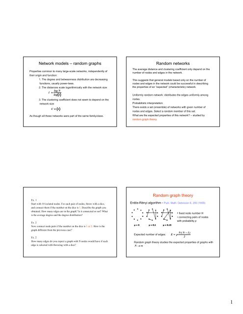
<strong>Network</strong> <strong>models</strong> – <strong>random</strong> <strong><strong>graph</strong>s</strong><br />
Properties common to many large-scale <strong>networks</strong>, independently of<br />
their origin and function:<br />
1. The degree and betweenness distribution are decreasing<br />
functions, usually power-laws.<br />
2. The distances scale logarithmically with the network size<br />
log N<br />
l ≈<br />
log k<br />
3. The clustering coefficient does not seem to depend on the<br />
network size<br />
C ∝ k<br />
As though all these <strong>networks</strong> were part of the same family/class.<br />
<strong>Random</strong> <strong>networks</strong><br />
The average distance and clustering coefficient only depend on the<br />
number of nodes and edges in the network.<br />
This suggests that general <strong>models</strong> based only on the number of<br />
nodes and edges in the network could be successful in describing<br />
the properties of an “expected” (characteristic) network.<br />
Uniformly <strong>random</strong> network: distributes the edges uniformly among<br />
nodes.<br />
Probabilistic interpretation:<br />
There exists a set (ensemble) of <strong>networks</strong> with given number of<br />
nodes and edges. Select a <strong>random</strong> member of this set.<br />
What are the expected properties of this network? – studied by<br />
<strong>random</strong> <strong>graph</strong> theory.<br />
Ex. 1<br />
Start with 10 isolated nodes. For each pair of nodes, throw with a dice,<br />
and connect them if the number on the dice is 1. Describe the <strong>graph</strong> you<br />
obtained. How many edges are in the <strong>graph</strong>? Is it connected or not? What<br />
is the average degree and the degree distribution?<br />
Ex. 2<br />
Now connect node pairs if the number on the dice is 1 or 2. How is the<br />
<strong>graph</strong> different from the previous case?<br />
Ex. 2<br />
How many edges do you expect a <strong>graph</strong> with N nodes would have if each<br />
edge is selected with throwing with a dice?<br />
<strong>Random</strong> <strong>graph</strong> theory<br />
Erdös-Rényi algorithm - Publ. Math. Debrecen 6, 290 (1959)<br />
Expected number of edges:<br />
• fixed node number N<br />
• connecting pairs of nodes<br />
with probability p<br />
N( N − 1 )<br />
E = p<br />
2<br />
<strong>Random</strong> <strong>graph</strong> theory studies the expected properties of <strong><strong>graph</strong>s</strong> with<br />
N → ∞<br />
1
The properties of <strong>random</strong> <strong><strong>graph</strong>s</strong> depend<br />
on p<br />
Properties studied:<br />
is the <strong>graph</strong> connected?<br />
does the <strong>graph</strong> contain a giant connected component?<br />
what is the diameter of the <strong>graph</strong>?<br />
does the <strong>graph</strong> contain cliques (complete sub<strong><strong>graph</strong>s</strong>)?<br />
Probabilistic formulation: what is the probability that a <strong>graph</strong> with<br />
N nodes and connection probability p is connected?<br />
Increase p from 0 to 1. Some of these properties appear suddenly,<br />
at a threshold p c (N)<br />
lim P<br />
N<br />
→∞<br />
N ,<br />
( Q ) =<br />
p<br />
0 if<br />
1 if<br />
p(N )<br />
→ 0<br />
p ( N )<br />
c<br />
p(N )<br />
→ ∞<br />
p ( N )<br />
c<br />
Ways of selecting<br />
n nodes from N<br />
Sub<strong><strong>graph</strong>s</strong> of a <strong>random</strong> <strong>graph</strong><br />
Consider a sub<strong>graph</strong> with n nodes and e edges.<br />
Expected number of of these sub<strong><strong>graph</strong>s</strong> in a <strong>graph</strong> with N nodes<br />
and connection prob. p<br />
We can permute<br />
n e n!<br />
the n nodes in any<br />
E( X ) = C<br />
N<br />
p<br />
a<br />
way we want...<br />
Probability of<br />
having e edges<br />
Isomorphic <strong><strong>graph</strong>s</strong>: there exists a<br />
one-to-one mapping of the nodes<br />
in such a way that if (and only if)<br />
node i and j are connected in one<br />
then their images i’ and j’ are also<br />
Connected.<br />
but identical<br />
(isomorphic) <strong><strong>graph</strong>s</strong><br />
do not count<br />
Special sub<strong><strong>graph</strong>s</strong><br />
Consider a sub<strong>graph</strong> with n nodes and e edges.<br />
Expected number of sub<strong><strong>graph</strong>s</strong> with n nodes and e edges in a<br />
<strong>graph</strong> with N nodes and connection prob. p<br />
n e<br />
n e n! N p<br />
E( X ) = C<br />
N<br />
p ≅<br />
a a<br />
If the connection probability is a function of the number of the<br />
nodes, we can find the condition of having a non-vanishing<br />
number of sub<strong><strong>graph</strong>s</strong>.<br />
lim<br />
N→∞<br />
n / e<br />
p( N )N<br />
≠ 0<br />
Ex. Find the condition of having a non-vanishing number of<br />
trees, cycles and completely connected sub<strong><strong>graph</strong>s</strong>.<br />
Evolution of a <strong>random</strong> <strong>graph</strong><br />
Assume that the connection probability is a power-law of N,<br />
Assume that z increases from − ∞ to 0<br />
Look for trees, cycles (circuits) and cliques in the <strong>graph</strong>.<br />
Appearance thresholds:<br />
The <strong>graph</strong> contains cycles of any length if z ≥ −1<br />
z<br />
p = cN<br />
2
Clusters in a <strong>random</strong> <strong>graph</strong><br />
Node degrees in <strong>random</strong> <strong><strong>graph</strong>s</strong><br />
−1<br />
• For p < N the <strong>graph</strong> contains only isolated trees.<br />
−1<br />
• If p = cN with c < 1 the <strong>graph</strong> has isolated trees and cycles.<br />
−1<br />
•At p = cN with c = 1 a giant connected component appears.<br />
• The size of the giant connected component approaches N rapidly<br />
as c increases.<br />
S = (<br />
f ( 1 )<br />
−<br />
f ( c ))N<br />
P(k)<br />
0.10<br />
0.05<br />
<br />
0.00<br />
0.0 10.0 20.0 30.0<br />
k<br />
ways to select k<br />
nodes from N-1<br />
• average degree: 2E<br />
k = ≅ pN<br />
N<br />
• degree distribution:<br />
P( k )<br />
≅ C<br />
probability of<br />
having k edges<br />
k k<br />
N −1−k<br />
N −1<br />
p ( 1 − p )<br />
probability of<br />
missing N-1-k<br />
edges<br />
• The <strong>graph</strong> becomes connected if<br />
lim ln<br />
p<br />
N<br />
N →∞<br />
/<br />
= ∞<br />
N<br />
Most of the nodes have approximately the same degree.<br />
The probability of very highly connected nodes is exponentially<br />
small.<br />
Distances in <strong>random</strong> <strong><strong>graph</strong>s</strong><br />
There is no local order in <strong>random</strong> <strong><strong>graph</strong>s</strong><br />
<strong>Random</strong> <strong><strong>graph</strong>s</strong> tend to have a tree-like topology with almost<br />
constant node degrees.<br />
Measure of local order:<br />
ni<br />
Ci<br />
≡<br />
k ( k − 1 ) / 2<br />
i<br />
i<br />
• nr. of first neighbors:<br />
• nr. of second neighbors:<br />
N 1<br />
≅ k<br />
• estimate maximum distance:<br />
N<br />
2<br />
≅ k<br />
2<br />
Since edges are independent and have the same probability p,<br />
ki<br />
( ki<br />
− 1 )<br />
n<br />
< k ><br />
i<br />
≅ p<br />
2 C ≅ p =<br />
N<br />
1<br />
l<br />
+ max<br />
∑<br />
l = 1<br />
k<br />
i<br />
= N<br />
log N<br />
l max<br />
=<br />
log k<br />
The clustering coefficient of <strong>random</strong> <strong><strong>graph</strong>s</strong> is small.<br />
This scaling was proven by Chung and Lu, Adv. Appl. Math 26,<br />
257 (2001).<br />
3
Are real <strong>networks</strong> like <strong>random</strong> <strong><strong>graph</strong>s</strong>?<br />
As quantitative data about real <strong>networks</strong> becomes available, we can<br />
compare their topology with that of <strong>random</strong> <strong><strong>graph</strong>s</strong>.<br />
Starting measures: N, for the real network.<br />
Determine l, C and P(k) for a <strong>random</strong> <strong>graph</strong> with the same N and .<br />
log N<br />
l rand<br />
≈<br />
log k<br />
P<br />
C rand<br />
= p =<br />
k k<br />
N −1−k<br />
rand<br />
( k ) ≅ C<br />
N −1<br />
p ( 1 − p )<br />
k<br />
N<br />
l log<br />
15<br />
10<br />
5<br />
Path length and order in real <strong>networks</strong><br />
log N<br />
k<br />
l rand<br />
=<br />
C<br />
log k<br />
rand<br />
=<br />
N<br />
food webs<br />
neural network<br />
power grid<br />
collaboration <strong>networks</strong><br />
WWW<br />
metabolic <strong>networks</strong><br />
Internet<br />
C/<br />
10 0<br />
10 -2<br />
food webs<br />
10 -4 neural network<br />
metabolic <strong>networks</strong><br />
power grid<br />
collaboration <strong>networks</strong><br />
10 -6 WWW<br />
Measure l, C and P(k) for the real network. Compare.<br />
0<br />
10 0 10 2 10 4 10 6 10 8 10 10<br />
N<br />
10 -8<br />
10 0 10 2 10 4 10 6 10 8<br />
N<br />
Real <strong>networks</strong> have short distances like <strong>random</strong> <strong><strong>graph</strong>s</strong> yet show<br />
signs of local order.<br />
The degree distribution of the WWW is a<br />
power-law<br />
Power-law degree distributions were found in<br />
diverse <strong>networks</strong><br />
Internet, router level<br />
Actor collaboration<br />
P<br />
out<br />
( k)<br />
≈ k<br />
P ( k)<br />
≈ k<br />
in<br />
−2.<br />
45<br />
−2.<br />
1<br />
P(<br />
k)<br />
≈ k<br />
P(k)<br />
−2.4<br />
P(<br />
k)<br />
≈ k<br />
−2.3<br />
R. Albert, H. Jeong, A.-L. Barabási, Nature 401, 130 (1999)<br />
A. Broder et al., Comput. Netw. 33, 309 (1999)<br />
0 1 2 3<br />
1 2 3<br />
10 10 10 10 10 10 10<br />
k<br />
R. Govindan, H. Tangmunarunkit, IEEE Infocom (2000)<br />
A.-L. Barabási, R. Albert, Science 286, 509 (1999)<br />
4
The power-law degree distribution<br />
indicates a heterogeneous topology<br />
P(k)<br />
0.10<br />
0.05<br />
log P(k)<br />
10 0<br />
10 -2<br />
10 -4<br />
Idea: generate <strong>random</strong> <strong><strong>graph</strong>s</strong> with<br />
a power-law degree distribution<br />
Fixed N P k = Ak<br />
− γ<br />
, ( ) , k < K<br />
<strong>Network</strong> assembly - <strong>random</strong> edges, but enforcing the right<br />
P(k)<br />
<br />
0.00<br />
0.0 10.0 20.0 30.0<br />
k<br />
10 -6<br />
10 0 10 1 10 2<br />
log k<br />
K<br />
∑<br />
k = 1<br />
P(<br />
k )<br />
1<br />
= 1,<br />
⇒ A =<br />
K<br />
k<br />
∑<br />
1<br />
−γ<br />
K<br />
∑1<br />
∑<br />
K<br />
< k >= ∑ kP( k ), ⇒ < k >=<br />
K<br />
k = 1<br />
1<br />
k<br />
k<br />
−γ<br />
+ 1<br />
−γ<br />
The average degree gives<br />
the characteristic scale (value)<br />
of the degree.<br />
Large variability,<br />
the average degree not informative,<br />
no characteristic scale for the degree<br />
Scale-free<br />
The number of edges increases as γ decreases.<br />
Constructing <strong><strong>graph</strong>s</strong> with<br />
a given degree distribution<br />
Configuration model:<br />
• choose a degree sequence N(k)=N P(k)<br />
• give the nodes k “stubs” according to N(k)<br />
• connect stubs <strong>random</strong>ly<br />
M. E. J. Newman, S. H. Strogatz, and D. J. Watts,<br />
Phys. Rev. E 64, 026118 (2001)<br />
Ex. Construct a <strong>graph</strong> with 10 nodes and degree sequence<br />
N(1)=4, N(2)=3, N(3)=2, N(4)=1.<br />
What is a necessary condition for the <strong>graph</strong> construction?<br />
Theory of general <strong>random</strong> <strong><strong>graph</strong>s</strong><br />
Looks at a characteristic member of the ensemble of <strong><strong>graph</strong>s</strong> with<br />
given degree distribution.<br />
Seeks the answers to the same questions as <strong>random</strong> <strong>graph</strong> theory<br />
• is the <strong>graph</strong> connected?<br />
• does the <strong>graph</strong> contain a giant component?<br />
• what is the diameter of the <strong>graph</strong>?<br />
• what is the clustering coefficient of the <strong>graph</strong>?<br />
The theoretical concept needed for the analysis is the generating<br />
function.<br />
One important result: A giant connected component exists if the<br />
<strong>graph</strong> is sufficiently heterogeneous. 2<br />
k k ≥ 2<br />
5
Connectivity of scale-free <strong>random</strong> <strong><strong>graph</strong>s</strong><br />
Given:<br />
−γ<br />
N , P(<br />
k)<br />
≈ k for k ≤ κ<br />
Graph properties depend on the degree exponent<br />
• giant cluster:<br />
• connected:<br />
γ ≤ 3.47<br />
γ ≤ 2<br />
W. Aiello, F. Chung, L. Lu, Proc. 32th ACM Theor. Comp., 171 (2000)<br />
M. E. J. Newman, S. H. Strogatz, D. J. Watts, Phys. Rev. E 64, 026118 (2001)<br />
γ<br />
Average path length of scale-free <strong>random</strong><br />
<strong><strong>graph</strong>s</strong><br />
<strong>Network</strong>:<br />
N , P(<br />
k)<br />
≈ k<br />
ln N + B<br />
Prediction: l sf<br />
= + 1 A , B = f ( γ , κ )<br />
A<br />
A(l-1)-B<br />
15<br />
10<br />
5<br />
food webs<br />
metabolic <strong>networks</strong><br />
Internet<br />
collaboration <strong>networks</strong><br />
WWW<br />
−γ<br />
0<br />
10 0 10 2 10 4 10 6 10 8 10 10<br />
N<br />
for<br />
k ≤ κ<br />
M. E. J. Newman, S. H. Strogatz, D. J. Watts, Phys. Rev. E 64, 026118 (2001)<br />
• qualitative agreement<br />
• worse than a <strong>random</strong><br />
<strong>graph</strong><br />
Clustering coefficient of scale-free<br />
<strong>random</strong> <strong><strong>graph</strong>s</strong><br />
2<br />
< k > ⎛ < k > − < k ><br />
C =<br />
⎜<br />
2<br />
N ⎝ < k ><br />
2<br />
2<br />
⎞<br />
⎟<br />
⎠<br />
The second term depends on the variance of the degree distribution.<br />
P )<br />
−γ<br />
( k ≈ k<br />
−( 3γ<br />
−7)/(<br />
γ −1)<br />
C ≈ N<br />
For γ < 7/3 C increases with N.<br />
M. E. J. Newman, SIAM Review 45, 167 (2003)<br />
Expectations:<br />
k ≥ 1 giant connected component, k ≥ ln N<br />
γ ≤ 3.47 giant connected component, γ ≤ 2<br />
connected<br />
connected<br />
6
Exponential <strong>random</strong> <strong><strong>graph</strong>s</strong><br />
“Exponential” does not refer to the degree distribution but to<br />
the model construction!<br />
This is a statistical method for generating a of <strong>graph</strong> with N<br />
nodes by specifying a distribution function over all <strong><strong>graph</strong>s</strong> with N nodes.<br />
1. Select a set of informative network measures (e.g. number of edges,<br />
number of triangles, degree distribution)<br />
2. Then select a network from the ensemble of all <strong><strong>graph</strong>s</strong> using the<br />
probability<br />
⎛ ⎞<br />
P(G ) ~ exp⎜<br />
− ∑ β<br />
iε<br />
i<br />
⎟<br />
⎝ i ⎠<br />
β i – parameters, ε i – network measures<br />
3. Estimate the coefficients such that an observed (real) network<br />
corresponds to the most likely <strong>graph</strong> in that ensemble – maximum<br />
likelihood estimation<br />
Markov <strong><strong>graph</strong>s</strong>: edges that do not share a node are independent<br />
Further reading: Frank & Strauss 1986, David Hunter’s webpage<br />
7