Mathcad - genfit.mcd

Nonlinear Regression II
Physics 258 - DS Hamilton 2004
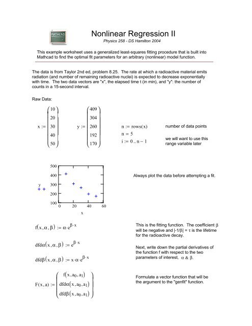
This example worksheet uses a generalized least-squares fitting procedure that is built into
Mathcad to find the optimal fit parameters for an arbitrary (nonlinear) model function.
The data is from Taylor 2nd ed, problem 8.25. The rate at which a radioactive material emits
radiation (and number of remaining radioactive nuclei) is expected to decrease exponentially
with time. The two data vectors are "x", the elapsed time t (in min), and "y": the number of
counts in a 15-second interval.
Raw Data:
x :=
⎛
⎜
⎜
⎜
⎜
⎜
⎝
10
20
30
40
50
⎞
⎟⎟
⎟
⎟
⎟
⎠
y :=
⎛
⎜
⎜
⎜
⎜
⎜
⎝
409
304
260
192
170
⎞
⎟⎟
⎟
⎟
⎟
⎠
n :=
n = 5
rows( x)
i := 0..
n − 1
number of data points
we will want to use this
range variable later
500
400
Always plot the data before attempting a fit.
y
300
200
100
0 20 40 60
x
( ) α e β ⋅x
f x, α , β
dfdα x, α , β
dfdβ x, α , β
F( x,
a)
( ) e β ⋅x
( ) := x⋅α
:=
:=
⎛
⎜
⎜
⎜
⎝
⋅
:=
( )
( , , a 1 )
( , )
f x, a 0 , a 1
dfdα x a 0
e β ⋅x
dfdβ x, a 0 a 1
⋅
⎞
⎟
⎟
⎟
⎠
This is the fitting function. The coefficient β
will be negative and |-1/β| = τ is the lifetime
for the radioactive decay.
Next, write down the partial derivatives of
the function f with respect to the two
parameters of interest, α & β.
Formulate a vector function that will be
the argument to the "genfit" function.

a :=
⎛
⎜
⎝
500
−0.5
⎞
⎟
⎠
Initial guess for the two parameters. This
is one reason to plot the data first.
⎛α
⎞ ⎜⎝ ⎟⎠ := genfit( x, y, a,
F)
β
Call the function "genfit" to find the
best-fit coefficients.
The solution is:
α = 505.3 β = −0.023
1
β
= −43.392 These are basically identical to those
found in the "minssd" example.
t := 0, 0.1..
60
Use this dummy variable to plot the fit so that it looks like a
smooth curve through 600 points.
600
500
y
( )
f t , α , β
400
300
200
100
0
0 10 20 30 40 50 60
x,
t
SSD :=
∑ ( y i − f ( x i , α , β ))2
i
SSD
= 10.1
n
This is the RMS difference between the data pints and
the fitting function.