The Fields of a Short, Linear Dipole Antenna If There Were No ...

The Fields of a Short, Linear Dipole Antenna
If There Were No Displacement Current
1 Problem
Kirk T. McDonald
Joseph Henry Laboratories, Princeton University, Princeton, NJ 08544
(July 5, 2006)
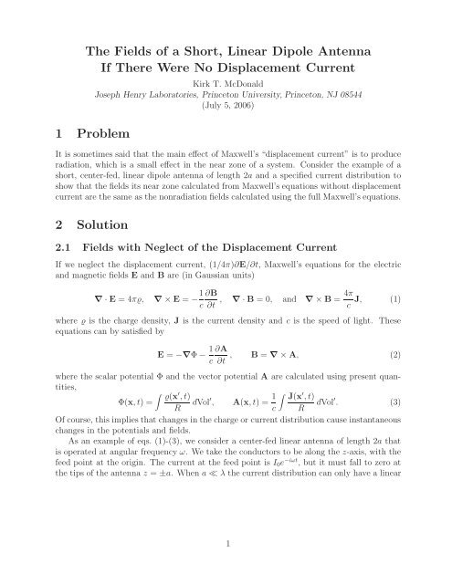
It is sometimes said that the main effect of Maxwell’s “displacement current” is to produce
radiation, which is a small effect in the near zone of a system. Consider the example of a
short, center-fed, linear dipole antenna of length 2a and a specified current distribution to
show that the fields its near zone calculated from Maxwell’s equations without displacement
current are the same as the nonradiation fields calculated using the full Maxwell’s equations.
2 Solution
2.1 Fields with Neglect of the Displacement Current
If we neglect the displacement current, (1/4π)∂E/∂t, Maxwell’s equations for the electric
and magnetic fields E and B are (in Gaussian units)
∇ · E =4πϱ, ∇ × E = − 1 ∂B
c ∂t , ∇ · B =0, and ∇ × B = 4π J, (1)
c
where ϱ is the charge density, J is the current density and c is the speed of light. These
equations can by satisfied by
E = −∇Φ − 1 ∂A
, B = ∇ × A, (2)
c ∂t
where the scalar potential Φ and the vector potential A are calculated using present quantities,
∫ ϱ(x ′ ,t)
Φ(x,t)=
R dVol′ , A(x,t)= 1 ∫ J(x ′ ,t)
c R dVol′ . (3)
Of course, this implies that changes in the charge or current distribution cause instantaneous
changes in the potentials and fields.
As an example of eqs. (1)-(3), we consider a center-fed linear antenna of length 2a that
is operated at angular frequency ω. We take the conductors to be along the z-axis, with the
feed point at the origin. The current at the feed point is I 0 e −iωt , but it must fall to zero at
the tips of the antenna z = ±a. Whena ≪ λ the current distribution can only have a linear
1

dependence on z, so its form must be 1
I(|z|

Far from the antenna the potentials (6) and (7) simplify to the forms
Φ ≈ I 0az
sin(ωt), and A
ckr0
3 z ≈ I 0a
cos(ωt), (9)
cr 0
where r 0 = √ ρ 2 + z 2 . The far-zone scalar potential is that of a dipole consisting of charges
±iI 0 /ω separated by distance a, and the vector potential is that due to a length a of current
I 0 , with both potentials oscillating at frequency ω.
The magnetic field has only a φ component, and varies only as cos(ωt),
B φ = − ∂A z
∂ρ = ρI [
0
ca cos(ωt) 1
r 1 − (z − a) + 1
r 2 − (z + a) − 2 ]
r 0 − z
= I 0
cρa (r 1 + r 2 − 2r 0 )cos(ωt) ≈ I 0a sin θ
cos(ωt), (10)
cr0
2
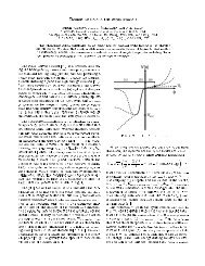
where the approximation holds for r 0 ≫ a, and the distances r 1 and r 2 are from the tips of
the antenna to the observation point, as shown in the figure below, where
r0 2 = ρ2 + a 2 , r1 2 = ρ2 +(z − a) 2 , r2 2 = ρ2 +(z + a) 2 . (11)
The ρ component of the electric field is
E ρ = − ∂Φ
∂ρ = − ρI [
]
0
cka sin(ωt) 1
r 1 (r 1 − (z − a)) + 1
r 2 (r 2 − (z + a)) − 2
r 0 (r 0 − z)
= − I [
0 z − a
+ z + a − 2z ]
sin(ωt) ≈ 3I 0a cos θ sin θ
sin(ωt), (12)
cρka r 1 r 2 r 0 ckr0
3
and the z component of the electric field is
E z = − ∂Φ
∂z − 1 ∂A z
= I {
0 1
c ∂t cka sin(ωt) + 1 − 2 r 1 r 2 r 0
−k 2 [r 1 + r 2 − 2r 0 +(z − a)ln(r 1 − z + a)+(z + a)ln(r 2 − z − a) − 2z ln(r 0 − z)] }
≈
I 0a
ck
( 3cos 2 θ − 1
r 3 0
+ k2
r 0
)
sin(ωt), (13)
3

where the approximation hold at large distances. The electric field varies only as sin(ωt).
The components of the electric field in spherical coordinates for r 0 ≫ a are
E r ≈ I 0a
ck
(
2
r 3 0
− k2
r 0
)
cos θ sin(ωt),
E θ ≈ I 0a
ck
(
1
r 3 0
+ k2
r 0
)
sin θ sin(ωt). (14)
For large r 0 the electric field, but not the magnetic field, has a term that falls off as 1/r 0 .
Since E and B are out of phase the time-average Poynting vector is zero, and there is
no (time-average) transport of energy away from the source when displacement current is
neglected.
In the near zone, where kr j ≪ 1forj =0, 1, 2 the nonzero field components can be
written
B φ (kr j ≪ 1) = I 0
cρa [r 1 + r 2 − 2r 0 ]cos(ωt), (15)
E ρ (kr j ≪ 1) = − I [
0 z − a
+ z + a − 2z ]
sin(ωt), (16)
cρka
r 0
E z (kr j ≪ 1) ≈ I 0
cka
r 1
r 2
[ 1
r 1
+ 1 r 2
− 2 r 0
]
sin(ωt). (17)
2.2 Near Fields When Displacement Current Is Included
This section follows sec. 2.3 of [1] as to the near fields of a linear dipole antenna of length
2a, withanassumed current distribution
sin[k(a −|z|)] cos ωt
I(z,t) =I 0 , (18)
sin ka
which is normalized such that I(z =0)=I 0 cos ωt.
The electric and magnetic fields can be calculated from the retarded vector potential,
which has only a z-component in this example,
A z (x,t)= 1 c
∫ a
−a
dz ′ I(z ′ ,t ′ = t − R/c)
R
= I 0e −iωt
c
∫ a
−a
dz ′
sin sin[k(a −|z ′ |)] eikR
R , (19)
where k =2π/λ = ω/c and R = |x − x ′ |. Then, the fields E and B are related by 2
B = ∇ × A,
and
[ ] i ∂E
kc ∂t = E = i ∇ × B. (20)
k
We evaluate the field components in a cylindrical coordinate system (ρ, φ, z) to find for
a small antenna with ka ≪ 1,
B ρ = 0, (21)
2 We note that the sequence of calculations in eqs. (19) and (20) could be interpreted as implying that the
conduction current I leads to the vector potential and the magnetic field, and then the curl of the magnetic
field leads to the “displacement current” (1/4π)∂E/∂t.
4

{ iI0 e −iωt [
(
B φ = −Re e ikr 1
+ e ikr 2
− 2e ikr 0
1 − k2 a 2 )]}
(22)
cρka
2
= I [
(
0
sin(kr 1 − ωt)+sin(kr 2 − ωt) − 2 1 − k2 a 2 )
]
sin(kr 0 − ωt) , (23)
cρka
2
B z = 0, (24)
{ iI0 e −iωt [ (z − a)e
ikr 1
E ρ = −Re
+ (z + (
a)eikr 2
− 2 zeikr 0
1 − k2 a 2 )]}
(25)
cρka r 1 r 2 r 0 2
= I [
0
(z − a) sin(kr 1 − ωt)
+(z + a) sin(kr (
2 − ωt)
− 2z 1 − k2 a 2 ) ]
sin(kr0 − ωt)
(26) ,
cρka
r 1
r 2
2 r 0
E φ = 0, (27)
{ iI0 e −iωt [ (
e
ikr 1
E z = Re
+ eikr 2
− 2 eikr 0
1 − k2 a 2 )]}
(28)
cka r 1 r 2 r 0 2
= − I [
0 sin(kr1 − ωt)
+ sin(kr (
2 − ωt)
− 2 1 − k2 a 2 ) ]
sin(kr0 − ωt)
. (29)
cka r 1
r 2 2 r 0
For completeness, we also display the field components in a spherical coordinate system
(r, θ, φ), noting that ρ = r 0 sin θ,
B r = 0, (30)
B θ = 0, (31)
{ iI0 e −iωt [
(
B φ = −Re e ikr 1
+ e ikr 2
− 2e ikr 0
1 − k2 a 2 )] }
sin θ
(32)
cr 0 ka
2
[
(
I 0
= sin(kr 1 − ωt)+sin(kr 2 − ωt) − 2 1 − k2 a 2 )
]
sin(kr 0 − ωt) sin θ, (33)
cr 0 ka
2
{ iaI0 e −iωt [ ]}
e
ikr 1
E r = Re
− eikr 2
(34)
cr 0 ka r 1 r 2
= − I [
0a sin(kr1 − ωt)
− sin(kr ]
2 − ωt)
, (35)
cr 0 ka r 1
r 2
{
iI0 e −iωt [
(r
2
E θ = −Re
0 − az)e ikr 1
+ (r2 0 + az)e ikr (
2
− 2r
cr0ka 2 0 e ikr 0
1 − k2 a 2 )]}
(36)
sin θ r 1 r 2 2
[
I 0
=
(r
cr0ka 2 0 2 − az) sin(kr 1 − ωt)
+(r0 2 + az) sin(kr 2 − ωt)
sin θ
r 1
r 2
(
−2r 0 1 − k2 a 2 )
]
sin(kr 0 − ωt) . (37)
2
E φ = 0, (38)
The radiation fields are most prominent in the far zone, where r = r 0 ≈ r 1 ≈ r 2 . In spherical
coordinates the only nonzero components to the radiation fields are 3
{ iI0 ka e i(kr }
0−ωt)
B φ = E θ = −Re
sin θ = I 0a sin(kr 0 − ωt)
sin θ. (39)
c
c r 0
r 0
3 Verification that eqs. (36) and (37) become eq. (39) in the far zone is a bit subtle. See [1].
5

The radiation fields depend on the small quantity ka, which permits us to identify the
radiation fields in the near zone, where they are only a small part of the total fields.
Close to the antenna, where kr j ≪ 1wehavecos(kr j ) ≈ 1 and sin(kr j ) ≈ kr j for
j =0, 1, 2. The nonzero field components (23), (26) and (29) in cylindrical coordinates
simplify to the forms close to the antenna:
B φ (kr j ≪ 1) ≈ I [
0 r1 + r 2 − 2r 0
cρ a
[ z − a
E ρ (kr j ≪ 1) ≈ − I 0
+ z + a
cρka r 1 r 2
E z (kr j ≪ 1) ≈ I [
0 1
+ 1 − 2 (
cka r 1 r 2 r 0
]
cos(ωt) − ka sin(ωt) , (40)
− 2z
r 0
(
1 − k2 a 2
2
1 − k2 a 2 )]
sin(ωt), (41)
2
)]
sin(ωt). (42)
Close to the antenna all of the electric field varies as sin(ωt), and so is 90 ◦ out of phase with
the drive current. The largest part of the magnetic field is in phase with the current, but
the radiation part of the magnetic field (which varies as ka) is90 ◦ out of phase with the
current, and is therefore in phase with the electric field. Furthermore, the radiation parts
of the electric and magnetic field have very similar magnitudes close to the antenna, even
though the total electric field is much larger than the total magnetic field here.
Thus, the assumed current distribution (4) generates radiation fields in its near zone that
are similar in character to the radiation fields in the far zone: E rad ≈ B rad in magnitude an
phase, and directed at right angles to one another.
The nonradiation (“reactive”) parts of the fields in the near zone are
B φ (kr j ≪ 1, non rad) ≈ I 0
cρa [r 1 + r 2 − 2r 0 ]cos(ωt), (43)
E ρ (kr j ≪ 1, non rad) ≈ − I [
0 z − a
+ z + a − 2z ]
sin(ωt), (44)
cρka
r 0
E z (kr j ≪ 1, non rad) ≈ I 0
cka
r 1
r 2
[ 1
r 1
+ 1 r 2
− 2 r 0
]
sin(ωt), (45)
which are the same as those found in eqs. (15)-(17) by ignoring the displacement-current in
Maxwell’s equations.
A Appendix: The Electric and Magnetic Fields are
NotJustRetardedStaticFields
It is well known that the electric and magnetic fields described by Maxwell’s equations can
be deduced from the retarded potentials [2],
∫ ϱ(x ′ ,t ′ )
Φ(x,t)=
R dVol′ , A(x,t)= 1 ∫ J(x ′ ,t ′ )
dVol ′ . (46)
c R
which have the form of the static potentials and current distributions evaluated at the retarded
time t ′ = t − R/c, whereR = |x − x ′ |, rather than at the present time. However, it
6

does NOT follow that the electric and magnetic fields have the form of the static fields with
the charge and current distributions evaluated at the retarded time. Instead, the fields can
be calculated from the charge and current distributions according to 4
∫ [ϱ] ˆR
E = dVol ′ + 1 ∫ ([J] · ˆR) ˆR +([J] × ˆR) × ˆR
dVol ′ + 1 ∫ ( [J] ˙ × ˆR) × ˆR dVol ′ , (47)
R 2 c
R 2 c 2 R
and
B = 1 ∫ [J] × ˆR
dVol ′ + 1 ∫
[J] ˙ × ˆR
c R 2 c 2 R dVol′ , (48)
where ˆR = R/R =(x − x ′ )/ |x − x ′ |, and quantities inside brackets, [...], are evaluated at
the retarded time t ′ = t − R/c.
If the charge and current distributions are oscillatory with a single frequency ω, wecan
write
ϱ(x,t)=ϱ 0 (x)e −iωt , and J(x,t)=J 0 (x)e −iωt . (49)
The oscillatory factor e −iωt when evaluated at the retarded time t ′ = t − R/c becomes the
waveform e −iω(t′ −R/c) = e i(kR−ωt) ,wherek = ω/c =2π/λ. In this case, the electric and
magnetic fields can be written as
∫ ϱ0 ˆR
E =
R 2 ei(kR−ωt) dVol ′ + 1 ∫ (J0 · ˆR) ˆR +(J 0 × ˆR) × ˆR e i(kR−ωt) dVol ′
c
R 2
− ik ∫ (J0 × ˆR) × ˆR e i(kR−ωt) dVol ′ , (50)
c R
and
B = 1 ∫ J0 × ˆR e i(kR−ωt) dVol ′ − ik ∫ J0 × ˆR
c R 2
c R ei(kR−ωt) dVol ′ , (51)
The first term of eqs. (47) and (50) could be called the retarded Coulomb field, and the
first term of eqs. (48) and (51) could be called the retarded Biot-Savart field. Both of these
terms vary as the inverse square of the distance between the source and observer, and so
they are important in the near zone and negligible in the far zone.
It is perhaps surprising that the electric field has a second term that varies inversely
with the square of the distance, and which is due to the current distribution rather than the
charge distribution. 5 This term is an indirect effect of Maxwell’s “displacement current”,
and in examples such as the present it makes a significant contribution to the difference
between the actual near-zone fields and those approximated by neglect of the “displacement
current”.
The last terms of eqs. (47)-(48) and (50)-(51) vary inversely with the distance between
the source and observer. These terms are the radiation fields, which are the most significant
additions to the fields when the “displacement current” is included in Maxwell’s equations.
The form of these terms shows that each current element whose time derivative is nonzero
creates electric and magnetic radiation fields that are 90 ◦ out of phase with respect to the
current, and which are equal in magnitude and at right angles to one another.
4 Equations (47) and (48) first appeared in [3].
5 The second term of the electric field vanishes for steady currents. See sec. 3 of [4]. While this term is
expressed as a function only of the conduction currents, it would be absent if the “displacement current”
were not present in Maxwell’s equations.
7

References
[1] K.T. McDonald, Radiation in the Near Zone of a Center-Fed Linear Antenna (June 21,
2003), http://puhep1.princeton.edu/~mcdonald/examples/linearantenna.pdf
[2] L. Lorenz, On the Identity of the Vibrations of Light with Electrical Currents, Phil.
Mag. 34, 287-301 (1867),
http://puhep1.princeton.edu/~mcdonald/examples/EM/lorenz_pm_34_287_67.pdf
[3] W.K.H. Panofsky and M. Phillips, Classical Electricity and Magnetism, 2nd ed.
(Addison-Wesley, Reading, MA, 1962).
[4] K.T. McDonald, The Relation Between Expressions for Time-Dependent Electromagnetic
Fields Given by Jefimenko and by Panofsky and Phillips (Dec. 6, 1996),
http://puhep1.princeton.edu/~mcdonald/examples/jefimenko.pdf
8