Reactance of Small Antennas - Princeton University

1 Problem
Reactance of Small Antennas
Kirk T. McDonald
Joseph Henry Laboratories, Princeton University, Princeton, NJ 08544
(June 3, 2009; updated September 11, 2012)
Estimate the capacitance and inductance of a short, center-fed, linear dipole antenna whose
arms each have length h and radius a. Also estimate the inductance of a small loop antenna
of major radius b and minor radius a.
For completeness, consider also the real part, its so-called radiation resistance, of the
antenna impedance in the approximation of perfect conductors.
2 Solution
2.1 Short, Center-Fed, Linear Dipole Antenna
This solution follows sec. 10.3 of [1].
2.1.1 Capacitance
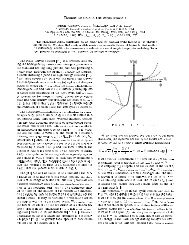
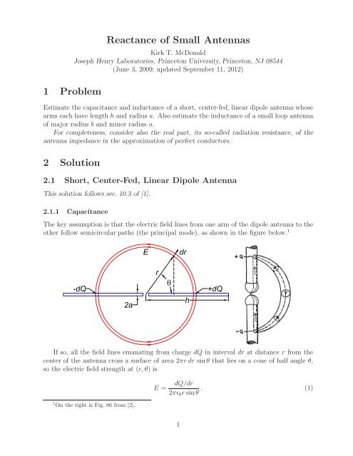
The key assumption is that the electric field lines from one arm of the dipole antenna to the
other follow semicircular paths (the principal mode), as shown in the figure below. 1
If so, all the field lines emanating from charge dQ in interval dr at distance r from the
center of the antenna cross a surface of area 2πr dr sin θ that lies on a cone of half angle θ,
so the electric field strength at (r, θ) is
1 On the right is Fig. 86 from [2].
E =
dQ/dr
2πɛ 0 r sin θ . (1)
1

The voltage difference between the two arms of the antenna is 2
∫ π/2
ΔV =2 Er dθ = dQ/dr ∫ π/2 dθ
θ min πɛ 0 a/r sin θ = dQ/dr ln[tan(θ/2)] π/2
a/r
πɛ = dQ/dr ln(2r/a). (2)
0 πɛ 0
This voltage difference should be independent of position along the antenna. 3 The charge
distribution dQ/dr is indeed constant to a good approximation for short dipole antennas,
but the factor ln(2r/a) =− ln(θ min /2) is constant only for a biconical dipole antenna (as
much favored theoretically by Schelkunoff). A reasonable approximation for a linear dipole
antenna is to use r = h/2 as a representative length in eq. (2), which leads to the estimate
ΔV ≈ dQ/dr ln(h/a). (3)
πɛ 0
The corresponding capacitance per unit length along the antenna is
dC
dr ≈ πɛ 0
ln(h/a) , (4)
and the total capacitance is
C ≈
πɛ 0h
ln(h/a) . (5)
This estimate ignores the contribution to the capacitance of roughly πɛ 0 a 2 /d associated with
the electric field in the gap d between the terminals of the antenna, as is reasonable when
d ≈ a since then ln(h/a) ≪ h/a ≈ dh/a 2 .
2.1.2 Inductance
For a quick estimate of the inductance of the antenna we note when the arms carry current
I the magnetic field near the conductors varies with distance as
B ≈ μ 0I
2πr . (6)
The magnetic flux associated with the linear antenna is
∫ h
Φ=LI ≈ h Bdr≈ μ 0hI
a 2π ln h a , (7)
where we note that the current drops from I to0overlengthh of each arm. Then, our
rough estimate of the inductance L is
L ≈ μ 0h
2π ln h a . (8)
2 In general the electric field is related to the scalar and vector potentials by E = −∇V − ∂A/∂t =
−∇V − iωA, assuming a time dependence of the form e iωt . Then, ∫ 2
1 E · dl = V 1 − V 2 − iω ∫ 2
1 A · dl.
However, close to a small linear dipole antenna the electric field is much larger than the magnetic field (see,
for example, [3]), and the contribution of the vector potential to the electric field in negligible in this region.
3 The vanishing of the tangential component of the electric field along the (ideal) conductor implies that
this conductor is an equipotential only if the vector potential can be neglected. For examples where this
does not hold, see [4, 5].
2

2.1.3 Reactance
The reactance of a short linear antenna (h ≪ λ) is largely due to its capacitance,
X small linear = ωL − 1
ωC ≈− 1
ckC ≈−ln(h/a) πɛ 0 ckh = −Z 0 ln(h/a)
π kh
where (c =1/ √ ɛ 0 μ 0 being the speed of light in vacuum)
√
μ0
Z 0 = = μ
ɛ 0 c = 1
0 ɛ 0 c
= − Z 0
π 2
λ
ln(h/a), (9)
2h
= 377 Ω. (10)
The reactance (9) falls with increasing length h of the arms of the antenna, and vanishes
when
ω = √ 1
√
2π 1
≈ LC μ 0 h πɛ 0 h = √ 2 c √
2πc
2λ
= kc =
h λ , i.e., h ≈ 2π = λ
4.44 . (11)
Thus, the rough estimates (5) and (8) of C and L for a linear antenna give a fairly good
prediction of “resonance” when half-length h ≈ λ/4.
2.1.4 Relation between Reactance and “Free Oscillation”
As an aside, we note that frequencies at which the terminal reactance vanishes correspond
to those of “free oscillation of the antenna (with its terminals shorted).
In a “free oscillation” 4 radiation is ignored and the (near) fields are standing waves that
obey the Helmholtz equation, (∇ 2 + k 2 )ψ =0,whereψ is any scalar component of the
electric and magnetic fields. Electromagnetic energy is stored in the (near) fields, which
oscillates between “electric” and “magnetic” terms, there being no exchange of energy with
the perfect conductor.
For driven oscillations of a conductor, a nonzero terminal reactance implies an exchange
of energy between the energy/voltage source and the (near) electromagnetic fields.
Thus, if the reactance in nonzero at some frequency, that frequency cannot correspond to
a “free oscillation” (for which there is no exchange of energy between fields and conductors).
2.2 Small Loop Antenna
2.2.1 Inductance
One definition of a small loop antenna is that the spatial variation of the current around the
loop can be neglected. In this case the inductance is essentially that of a circular loop/torus
of,say,majorradiusb and minor radius a, supposing that all the current in on the surface
because of the skin effect.
ForaquickestimatewenotewhentheloopcarriescurrentI the magnetic field near the
conductor varies with distance as
B ≈ μ 0I
2πr , (12)
4 “Free oscillations” of (perfect) conductors were perhaps first discussed in [6]. See also, [7].
3

so the magnetic flux linked by the loop is
and the inductance L is
∫ b
Φ=LI ≈ 2πb Bdr≈ μ 0 bI ln b
a
a , (13)
L ≈ μ 0 b ln b (
a = μ 0b ln 8b )
a − 2.08 . (14)
A more exact calculation using toroidal coordinates [8] shows that the number 2.08 = ln 8
in eq. (14) is actually 2 when b ≫ a.
2.2.2 Capacitance
A loop antenna has a small capacitance C associated with the gap between its terminal.
However, the capacitive reactance 1/iωC is negligible in practice, so we skip estimating the
capacitance C. 5
2.2.3 Reactance
The reactance of a small loop antenna is essentially that due to its inductance,
X small loop ≈ ωL ≈ μ 0 ωb ln b a = μ 0ckb ln b a = Z 2πb
0
λ ln b a . (15)
A
Appendix: Radiation Resistance of Small Antennas
For completeness, we include the well-known calculations of the radiation resistance R rad of
small antennas, noting that the time-average radiated power P is related to the peak current
I 0 at the antenna terminals by
P = I 2 0R rad
2
= μ 0 |¨p| 2
12πc = μ 0 ω 4 |p 0 | 2
, i.e., R rad = μ 0 ω 4 |p 0 | 2
, (16)
12πc
6πcI0
2
where p 0 is the peak electric dipole moment of the antenna (or p 0 = m 0 /c in case the antenna
has magnetic dipole moment m).
A.1 Short Linear Antenna
A linear antenna (of half length h, alongthez-axis) has electric dipole moment p related to
its linear charge density ρ by
∫ h
p = ρz dz. (17)
−h
5 An estimate of the terminal capacitance is given as a/2 in eq. (5) of [9]. A very different estimate is
given in sec. 10-12 of [1], assuming that it is meaningful to consider the loop to be a capacitor consisting
of two half loops; however, the current around a small loop is uniform, so there is no charge distribution
around the loop, except at the terminals, and the estimate of [1] seems inappropriate.
4

The charge density is related to the current distribution
I(z,t) ≈ I 0 (1 −|z| /h) e iωt , (18)
by the continuity equation,
˙ρ = − dI
dz ≈±I 0
h eiωt , (19)
so that
ρ = ∓ iI 0
ωh eiωt , (20)
and
p 0 = − iI 0h
(21)
ω
from eq. (17). Then, according to eq. (16) the radiation resistance is, recalling eq. (10),
R rad = μ 0 ω 4 |p 0 | 2
6πcI 2 0
= μ 0 ω 2 h 2
6πc
= πμ 0 c (2h) 2
6
= πZ 0
6
(2h) 2
λ 2 . (22)
The approximation (19) is not very accurate for “resonance” with h ≈ λ/4, for which
eq. (22) gives R rad,resonance ≈ 377π/24 = 49 Ω rather than 71 Ω.
For an (“unmatched”) small linear antenna with terminal impedance Z ≈ iX and reactance
X given by eq. (9), the time-average radiated power when driven by a voltage source
V 0 is, noting that I 0 = |V 0 /Z|,
P linear,unmatched = V 0 2R
rad
2 |Z| 2 ≈ V 2
2X 2
0 R rad
≈
π 5 V0
2 (2h) 4
12Z 0 ln 2 (h/a) λ 4 . (23)
If the small linear antenna is “matched” to a line of (real) impedance Z line (≫ R rad )then
P linear,matched = V 2
0 R rad
2Z 2 line
≈ πV 0 2Z
0 (2h) 2
12Zline
2 λ 2 . (24)
A.2 Small Loop Antenna
A small loop antenna (of radius b) has azimuthally symmetric current I(φ, t) =I 0 e −iωt ,such
that the peak magnetic dipole moment is
and radiation resistance
m 0 = πb 2 I 0 , (25)
R rad = μ 0ω 4 |m 0 | 2
= πμ 0ω 4 b 4
= πμ 0c (2πb) 4
6πc 3 I0
2 6c 3 6 λ 4 = πZ 0 (2πb) 4
6 λ 4 . (26)
For an (“unmatched”) small loop antenna with reactance X given by eq. (15) the timeaverage
radiated power when driven by a voltage source V 0 is
P loop,unmatched ≈ V 2
0 R rad
2X 2
5
≈
πV0
2 (2πb) 2
12Z 0 ln 2 (b/a) λ 2 . (27)

If the small loop antenna is “matched” to a line of impedance Z line then
P loop,matched = V 2
0 R rad
2Z 2 line
≈ πV 0 2 Z 0 (2πb) 4
12Zline
2 λ 4 . (28)
Thus, a “matched,” small loop antenna of circumference 2πb radiates much less power than
a “matched,” small linear antenna of total length 2h =2πb. 6
References
[1] S.A. Schelkunoff and H.T. Friis, Antennas, Theory and Practice (Wiley, New York,
1952),
http://puhep1.princeton.edu/~mcdonald/examples/EM/schelkunoff_friis_antennas_c10.pdf
[2] H. Poincaré and F.K. Vreeland, Maxwell’s Theory and Wireless Telegraphy (McGraw,
New York, 1904),
http://puhep1.princeton.edu/~mcdonald/examples/EM/poincare_vreeland_04.pdf
[3] K.T. McDonald, Radiation in the Near Zone of a Hertzian Dipole (April 22, 2004),
http://puhep1.princeton.edu/~mcdonald/examples/nearzone.pdf
[4] K.T. McDonald, What Does an AC Voltmeter Measure? (March 16, 2008),
http://puhep1.princeton.edu/~mcdonald/examples/voltage.pdf
[5] K.T. McDonald, Lewin’s Circuit Paradox (May 7, 2010),
http://puhep1.princeton.edu/~mcdonald/examples/lewin.pdf
[6] M. Abraham, Die electrischen Schwingungen um einem stabförmigen Leiter, behandelt
nach der Maxwell’schen Theorie, Ann. Phys. 66, 435 (1898),
http://puhep1.princeton.edu/~mcdonald/examples/EM/abraham_ap_66_435_98.pdf
[7] Lord Rayleigh, On the Electrical Vibrations associated with thin terminated Conducting
Rods, Phil. Mag. 8, 104 (1904),
http://puhep1.princeton.edu/~mcdonald/examples/EM/rayleigh_pm_8_105_04.pdf
[8] V. Fock, Skin-Effekt in einem Ringe, Phys.Zeit.Sow.U.1, 215 (1932),
http://puhep1.princeton.edu/~mcdonald/examples/EM/fock_phys_z_sow_u_1_215_32.pdf
[9] K.T. McDonald, Radiation by an AC Voltage Source (Jan. 9, 2005),
http://puhep1.princeton.edu/~mcdonald/examples/acsource.pdf
6 An “unmatched,” small loop antenna of circumference 2πb radiates more power than an “unmatched,”
small linear antenna of total length 2h =2πb provided 2πb < ∼ λ/10, but the radiated power is quite small.
6