Electromagnetic Fields of a Small Helical Toroidal Antenna 1 ...

1 Problem
Electromagnetic Fields of a
Small Helical Toroidal Antenna
Kirk T. McDonald
Joseph Henry Laboratories, Princeton University, Princeton, NJ 08544
(December 8, 2008)
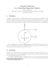
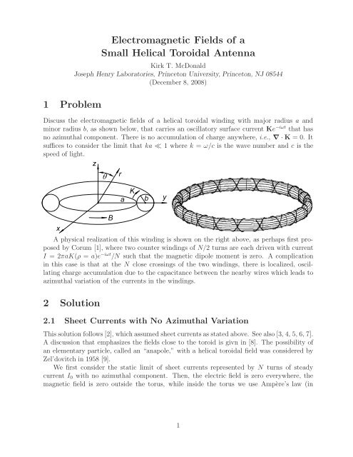
Discuss the electromagnetic fields of a helical toroidal winding with major radius a and
minor radius b, as shown below, that carries an oscillatory surface current Ke −iωt that has
no azimuthal component. There is no accumulation of charge anywhere, i.e., ∇ · K =0. It
suffices to consider the limit that ka ≪ 1wherek = ω/c is the wave number and c is the
speed of light.
A physical realization of this winding is shown on the right above, as perhaps first proposed
by Corum [1], where two counter windings of N/2 turns are each driven with current
I =2πaK(ρ = a)e −iωt /N such that the magnetic dipole moment is zero. A complication
in this case is that at the N close crossings of the two windings, there is localized, oscillating
charge accumulation due to the capacitance between the nearby wires which leads to
azimuthal variation of the currents in the windings.
2 Solution
2.1 Sheet Currents with No Azimuthal Variation
This solution follows [2], which assumed sheet currents as stated above. See also [3, 4, 5, 6, 7].
A discussion that emphasizes the fields close to the toroid is givn in [8]. The possibility of
an elementary particle, called an “anapole,” with a helical toroidal field was considered by
Zel’dovitch in 1958 [9].
We first consider the static limit of sheet currents represented by N turns of steady
current I 0 with no azimuthal component. Then, the electric field is zero everywhere, the
magnetic field is zero outside the torus, while inside the torus we use Ampère’s law (in
1

Gaussian units) to find
⎧
⎪⎨ 2NI 0 ˆφ/cρ (inside torus),
B static =
⎪⎩ 0 (outside torus),
(1)
where ρ = √ x 2 + y 2 .
The fact that both the static electric and magnetic vanish outside the torus implies that
all multiple moments vanish for a conventional multipole expansion in this region. However,
the vector potential is certainly nonzero inside the torus, so that continuity of the vector
potential at its surface implies that the vector potential is nonzero outside the torus as well. 1
To find the vector potential, and the electric and magnetic field, in the case of oscillating
currents in the windings, we follow a method due to Hertz. The electric and magnetic fields
E and B can be derived from the scalar and vector potentials V and A according to
E = −∇V − 1 ∂A
, B = ∇ × A, (2)
c ∂t
in Gaussian units. We work in the Lorentz gauge where the potentials satisfy the auxiliary
condition
∇ · A = − 1 ∂V
c ∂t . (3)
The potentials then obey the wave equations
∇ 2 A − 1 ∂ 2 A
c 2 ∂t = −4π 2 c J, ∇2 V − 1 ∂ 2 V
= −4πϱ, (4)
c 2 ∂t2 where ϱ and J are the charge and current densities of the sources of the waves. Formal
solutions for the (retarded) vector potential have been given by Lorenz,
A(r,t)= 1 c
∫
J(r ′ ,t ′ = t − R/c)
dVol ′ ,
R
∫
V(r,t)=
ϱ(r ′ ,t ′ = t − R/c)
dVol ′ , (5)
R
where R = |r − r ′ |.
There is nowhere any accumulation of charge in the present problem, so that ϱ =0and
hence the scalar potential V is zero as well. In this case, the Lorentz gauge condition (3)
tells us that
∇ · A =0, (6)
so that the vector potential can be written as the curl of another vector, which we will call
Z M ,themagnetic Hertz vector: 2 A = ∇ × Z M . (7)
From the wave equation (4) for the vector potential, we have
∇ 2 A = ∇ 2 (∇ × Z M )=∇ ×∇ 2 Z M = 1 c 2 ∂ 2 A
∂t 2
− 4π c J = ∇ × 1 c 2 ∂ 2 Z M
∂t 2 − 4π c J (8)
1 Aharonov and Bohm [10] have discussed quantum phenomena in the regions of zero magnetic field but
nonzero vector potential.
2 For additional discussion of electric and magnetic Hertz vectors and scalars, see the Appendix of [11].
2

If we write the current density as
J = c∇ × M, (9)
in terms of a magnetization density M, the magnetic Hertz vector satisfies the wave equation
∇ 2 Z M − 1 ∂ 2 Z M
= −4πM. (10)
c 2 ∂t 2
This justifies the alternative terminology that the magnetic Hertz vector is a polarization
potential, with the formal solution
∫
Z M (r,t)=
M(r ′ ,t ′ = t − R/c)
dVol ′ . (11)
R
If we regard the static magnetic field (1) inside the torus as due to a magnetization
density M rather than a conduction current density J or K, thenH = B − 4πM =0,sothe
required magnetization is
M static = B static
4π
⎧
⎪⎨ NI 0 ˆφ/2πcρ (inside torus),
=
⎪⎩ 0 (outside torus).
In the case of an oscillating current I 0 e −iωt , the equivalent oscillating magnetization is
(12)
M(ρ, t) =M static (ρ)e −iωt . (13)
Using this in eq. (11), the magnetic Hertz vector is given by
∫ Mstatic (ρ ′ )e i(kR−ωt)
Z M (r,t)=
dVol ′ . (14)
R
For an approximate solution, we use the relations
R ≈ r − ˆr · r ′ ,
where the term in 1/r 2 improves the accuracy at small r. Then, 3
Z M (r,t) ≈ ei(kr−ωt)
r
∫
≈ NI 0 e i(kr−ωt)
2πc r
1
R ≈ 1 (
1+ˆr · )
r′
, (15)
r r
( )
M static (ρ ′ )e −ikˆr·r′ 1+ r′ · ˆr
dVol ′
r
∫ φ
′ [ ( ) ]
1
1+
ρ ′ r − ik ˆr · r ′ dVol ′ (16)
We evaluate integral (16) for r in spherical coordinates (r, θ, φ) but r ′ in cylindrical coordinates
(ρ, φ, z), and for an observer at distance r ≫ a from the origin. In rectangular
coordinates, ˆr = (sinθ cos φ, sin θ sin φ, cos θ), r ′ = (ρ ′ cos φ ′ ,ρ ′ sin φ ′ ,z ′ )and ˆφ ′ =
3 Expanding the factor e ik·r′ to first order in r ′ in the Hertz vector Z M corresponds to expanding this
factor to second order in the vector potential A, which corresponds to keeping (magnetic) quadrupole terms
in the current density distribution.
3

− cos φ ′ ˆx +sinφ ′ ŷ,sothat
Z M (r ≫ a, t) ≈ NI 0 e i(kr−ωt) ∫ − cos φ′ ˆx +sinφ ′ ŷ
×
2πc r
ρ ′ [ ( )
]
1
× 1+
r − ik [ρ ′ (cos φ ′ sin θ cos φ +sinφ ′ sin θ sin φ)+z ′ cos θ] dVol ′
= NI 0V
4πc
= NI 0V
4πc
e i(kr−ωt)
r
e i(kr−ωt)
where V =2π 2 ab 2 is the volume of the torus.
The vector potential is
A(r ≫ a, t)=∇ × Z M ≈ NI 0V
4πc
r
( 1
r − ik )
sin θ (− cos φ ˆx +sinφ ŷ)
( 1
r − ik )
sin θ ˆφ, (17)
e i(kr−ωt) [
r
( 1
2
r − ik 2 r
)
cos θ ˆr +
The static vector potential is obtained by setting ω and k to zero,
( 1
r 2 − ik r − k2 )
sin θ ˆθ
]
.
(18)
A static (r ≫ a) ≈ NI 0V
4πcr 3 (2 cos θ ˆr +sinθ ˆθ) = 3(m T · ˆr)ˆr − m T
r 3 , (19)
where
m T = NI 0V ẑ. (20)
4πc
That is, the static vector potential outside the torus has the form of the magnetic field of
a magnetic dipole m T given by eq. (20), although the actual magnetic dipole moment of
the toroidal winding is zero. The quantity m T of eq. (20) has been called the toroid dipole
moment [5] because if this moment oscillates it generates an electric field formally similar to
that of an oscillating electric dipole (see eq. (21)). However, the moment (20) is the result
of weighting the current density J by two powers of distance, rather than by one, and so is
an aspect of the magnetic quadrupole moment of the current density.
The electric and magnetic fields outside the torus are
E(r ≫ a, t) = − 1 c
≈
∂A
∂t = ikA
ik NI 0V
4πc
e i(kr−ωt) [
r
(
1
2
r − ik 2 r
) (
1
r − ik ) ]
2 r − k2
cos θ ˆr +
sin θ ˆθ
= ik 3 ei(kr−ωt)
(ˆr × m T ) × ˆr +(ik + k 2 r)e i(kr−ωt) 3(m T · ˆr)ˆr − m T
, (21)
r
r 3
B(r ≫ a, t) = ∇ × A ≈−ik NI 0V e i(kr−ωt) (
1
4πc r r + ik )
2 r + k2 sin θ ˆφ
(
= ik 3 1 − 1
ikr + 1 ) e
i(kr−ωt)
ˆr × m
k 2 r 2 T . (22)
r
4

Both E and B vanish outside the torus in the static limit k = 0. The radiation fields are
e i(kr−ωt)
E rad,θ = B rad,φ = −ik 3 NI 0V
sin θ. (23)
4πc r
The fields (21)-(22) have the same form as those for a small oscillating electric dipole, except
that they are multiplied by an additional factor of k. And indeed, in a systematic multipole
expansion of the sources of vector electromagnetic fields (see, for example, sec. 9.10 of [12]) an
oscillating magnetization can contribute to the electric dipole moment, but with an additional
factor of k compared to the part of the electric dipole moment due to the electric charge
distribution.
The time-average radiated power has the angular distribution
dP rad
dΩ = 1
8πc
and the time-average radiated power is
where the radiation resistance R rad is given by
R rad = 1 3c
( NVk
3
4π
( NI0 Vk 3 ) 2
sin 2 θ, (24)
4π
P rad = 1 2 R radI 2 0, (25)
) 2
= π2 (
Nk 3 ab 2) 2 16π 8 ( ) Nab
2 2 ( ) Nab =
12c
3c λ 3 ≈ 1.5 × 10 6 2 2
λ 3 Ω. (26)
For example, if a = λ/10, b = λ/100 and N ≈ 580 turns, then R rad =50Ω.
Of course, the inductance L of such a winding is high. In SI units, the inductance is
L = μ 0N 2 b 2
2πa . (27)
For the above example, L ≈ 0.007 b henries for b in meters.
2.2 Counter-Wound Helical Toroidal Antenna
We give only a qualitative discussion of the counter-wound helical toroidal antenna, using
thecasethatN = 8 as an example.
As shown in the sketch below, the 8 = 2×4 turns can be thought of as forming 8 elongated
loops, each of which is formed from a half turn of each of the two counter windings, indicated
as diamonds on the left part of the figure. We suppose that the wires of the two windings
pass so close to one another that the capacitance of the 8 crossing points of the two windings
is very large. Then, there exist resonant frequencies at which the direction of the current in
each winding reverses at each crossing point, and the toroid dipole moment (20) vanishes.
5

Each of these loops has a magnetic moment m j that is perpendicular to the plane of each
loop, and which lies in the x-y plane, as shown on the right part of the figure.
At each of the 8 crossing points of the wires there is a large capacitance, and a corresponding
electric dipole moment p j that points towards (or away from) the center of the
toroid.
All electric and magnetic multipole moments of order less than N vanish, so the radiation
from the system is highly suppressed.
Foranobserveronthez axis, above the center of the antenna, the radiation electric field
vectors from the 8 magnetic moments m j and from the 8 electric dipole moments p j are
parallel to the x-y plane. The sum of the radiation electric fields is zero, and hence, there is
no radiation along the z axis.
An observer in the x-y plane sees very small electric field from the 8 electric dipole
moments, while the electric field from the 8 magnetic moments sums to a nonzero vertical
component.
The overall pattern of the radiation electric field is that it is largest, and approximately
independent of azimuth, in the x-y plane, while vanishing along the z direction. This is the
qualitative character of electric dipole radiation from an oscillating dipole moment directed
along the z-axis. However, it is ironic that when a counter-wound helical toroidal antenna
is operated at resonance, the toroid dipole moment vanishes, and this exotic antenna configuration
reduces to a circular array of “ordinary” electric and magnetic dipoles.
There exist some analytic studies in the literature for the case of small N [14, 15], but
some of their conclusion are at odds with the present analysis.
A
Appendix: The Chu Limit
One design goal of small antennas is a large bandwidth. In classic papers, Wheeler [17] and
Chu [18] noted that there is a limit to the bandwidth of an antenna that fits inside a sphere
6

of radius R ≪ λ that can be expressed as a lower limit on the Q of the antenna,
Q = ω 〈U near〉
〈P rad 〉
>
∼
1
4(kR) 3 , (28)
where 〈U near 〉 is the time-averaged energy stored in the non-propagating near electromagnetic
fields of the antenna and 〈P rad 〉 is the time-average radiated power. See also [19]. The bound
(28) is closely approached by a small linear dipole antenna of half-height R.
This argument is based on a decomposition of the fields of the antenna into multipole
moments. Since the counter-wound helical toroidal antenna has no nonzero electric or magnetic
multipole moments of the usual sort, it could be that this type of antenna can have
a Q smaller than the limit of eq. (28). We saw in sec. 2.1 that the fields outside the windings
of a small counter-wound helical toroidal antenna are essentially the same as those of a
small electric dipole antenna. Hence, the part of Q of a small counter-wound helical toroidal
antenna associated with the fields outside the windings is essentially the same as that of a
small electric dipole antenna, and therefore satisfies the bound (28). However, 〈U near 〉 also
includes the energy stored inside the windings,
〈U inside 〉 = 1 2 LI 2 0 , (29)
where L =2πN 2 b 2 /c 2 a in Gaussian units. This energy is much larger than that stored in
the near fields outside the windings. Then, recalling eqs. (25)-(26),
Q ≈ ωL = ω 2πN2 b 2 12c
R rad c 2 a π 2 N 2 a 2 b 4 k = 24
6 πk 5 a 2 b ≫ 1
3 4(ka) . (30)
3
Thus, a small counterwound helical toroidal antenna is a high-Q device and does not come
close to satisfying the Chu limit.
References
[1] J.F. Corum, Toroidal Helix Antenna, IEEE Ant. Prop. Int. Symp. 25, 832 (1987),
http://puhep1.princeton.edu/~mcdonald/examples/EM/corum_ieeeapsis_25_832_87.pdf
[2] N.J. Carron, On the fields of a torus and the role of the vector potential, Am. J.Phys.
63, 717 (1995),
http://puhep1.princeton.edu/~mcdonald/examples/EM/carron_ajp_63_717_95.pdf
[3] V.M. Dubovik and A.A. Cheshkov, Multipole expansion in classical and quantum field
theory and radiation, Sov.J.Part.Nucl.5, 318 (1975),
http://puhep1.princeton.edu/~mcdonald/examples/EM/dubovik_sjpn_5_318_75.pdf
[4] V.M. Dubovik and L.A. Tosunyan, Toroidal moments in the physics of electromagnetic
and weak interactions, Sov.J.Part.Nucl.14, 504 (1983),
http://puhep1.princeton.edu/~mcdonald/examples/EM/dubovik_sjpn_14_504_83.pdf
7

[5] V.M. Dubovik and V.V. Tugushev, Toroid Moments in Electrodynamics and Solid-State
Physics, Phys.Rep.187, 145 (1990),
http://puhep1.princeton.edu/~mcdonald/examples/EM/dubovik_pr_187_145_90.pdf
[6] G.N. Afanasiev, The electromagnetic fields of solenoids with time dependent currents,
J. Phys. A: Math. Gen. 23, 5755 (1990),
http://puhep1.princeton.edu/~mcdonald/examples/EM/afanasiev_jpa_23_5755_90.pdf
[7] I. Dumitriu and C. Vrejoiu, Some Aspects of Electromagnetic Multipole Expansions,
Rom. Rep. Phys. 60, 423 (2008),
http://puhep1.princeton.edu/~mcdonald/examples/EM/dumuitriu_rrp_60_423_08.pdf
[8] C.H. Page, External Field of an Ideal Toroid, Am.J.Phys.39, 1039 (1971),
http://puhep1.princeton.edu/~mcdonald/examples/EM/page_ajp_39_1039_71.pdf
On the External Magnetic Field of a Closed-Loop Core, Am.J.Phys.39, 1206 (1971),
http://puhep1.princeton.edu/~mcdonald/examples/EM/page_ajp_39_1206_71.pdf
[9] Y.B. Zel’dovitch, Electromagnetic Interaction with Parity Violation, Sov.Phys.JETP
6, 1184 (1958),
http://puhep1.princeton.edu/~mcdonald/examples/EM/zeldovich_jetp_6_1184_58.pdf
[10] Y. Aharonov and D. Bohm, Significance of Electromagnetic Potentials in the Quantum
Theory, Phys.Rev.115, 485 (1959),
http://puhep1.princeton.edu/~mcdonald/examples/QM/aharonov_pr_115_485_59.pdf
[11] K.T. McDonald, Radiation in the Near Zone of a Small Loop Antenna (June 7, 2004),
http://puhep1.princeton.edu/~mcdonald/examples/smallloop.pdf
[12] J.D. Jackson, Classical Electrodynamics, 3rd ed. (Wiley, New York, 1999).
[13] K.T. McDonald, Electrodynamics Problem Set 8 (2001),
http://puhep1.princeton.edu/~mcdonald/examples/ph501set8.pdf
[14] D.B. Miron, A Study of the CTHA Based on Analytical Models, IEEE Trans. Ant.
Prop. 49, 1130 (2001),
http://puhep1.princeton.edu/~mcdonald/examples/EM/miron_ieeetap_49_1130_01.pdf
[15] R.C. Hansen, Fields of the Contrawound Toroidal Helix Antenna, IEEE Trans. Ant.
Prop. 49, 1138 (2001),
http://puhep1.princeton.edu/~mcdonald/examples/EM/hansen_ieeetap_49_1138_01.pdf
[16] K.T. McDonald, Distortionless Transmission Line (Nov. 11, 1996),
http://puhep1.princeton.edu/~mcdonald/examples/distortionless.pdf
[17] H.A. Wheeler, Fundamental Limitations of Small Antennas, Proc. IRE 35, 1479 )1047),
http://puhep1.princeton.edu/~mcdonald/examples/EM/wheeler_pire_35_1479_47.pdf
[18] L.J. Chu, Physical Limitations of Omni-directional Antennas, J.Appl.Phys.19, 1163
(1948), http://puhep1.princeton.edu/~mcdonald/examples/EM/chu_jap_19_1163_48.pdf
8

[19] J.S. McLean, A Re-Examination of the Fundamental Limits on the Radiation Q of
Electrically Small Antennas, IEEE Trans. Ant. Prop. 44, 672 (1996),
http://puhep1.princeton.edu/~mcdonald/examples/EM/mclean_ieeetap_44_672_96.pdf
9