Physics 215A PS 4 Solutions
Physics 215A PS 4 Solutions
Physics 215A PS 4 Solutions

Create successful ePaper yourself
Turn your PDF publications into a flip-book with our unique Google optimized e-Paper software.
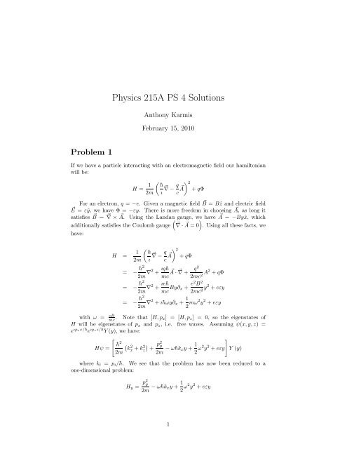
<strong>Physics</strong> <strong>215A</strong> <strong>PS</strong> 4 <strong>Solutions</strong><br />
Anthony Karmis<br />
February 15, 2010<br />
Problem 1<br />
If we have a particle interacting with an electromagnetic field our hamiltonian<br />
will be:<br />
H = 1 (¯h<br />
∇<br />
2m ı ⃗ − q ) 2<br />
A<br />
c ⃗ + qΦ<br />
For an electron, q = −e. Given a magnetic field B ⃗ = Bẑ and electric field<br />
⃗E = εŷ, we have Φ = −εy. There is more freedom in choosing A, ⃗ as long it<br />
satisfies B ⃗ = ∇ ⃗ × A. ⃗ Using the Landau( gauge, we ) have A ⃗ = −Byˆx, which<br />
additionally satisfies the Coulomb gauge ⃗∇ · A ⃗ = 0 . Using all these facts, we<br />
have:<br />
H =<br />
1<br />
(¯h<br />
∇<br />
2m ı ⃗ − q ) 2<br />
A<br />
c ⃗ + qΦ<br />
= − ¯h2<br />
2m ∇2 + ıq¯h A<br />
mc ⃗ · ⃗∇ +<br />
q2<br />
2mc 2 A2 + qΦ<br />
= − ¯h2<br />
2m ∇2 + ıe¯h<br />
mc By∂ x + e2 B 2<br />
2mc 2y2 + eεy<br />
= − ¯h2<br />
2m ∇2 + ı¯hωy∂ x + 1 2 mω2 y 2 + eεy<br />
with ω = eB<br />
mc . Note that [H, p x] = [H, p z ] = 0, so the eigenstates of<br />
H will be eigenstates of p x and p z , i.e. free waves. Assuming ψ(x, y, z) =<br />
e ıpxx/¯h e ıpzz/¯h Y (y), we have:<br />
[<br />
]<br />
¯h 2 (<br />
Hψ = k<br />
2<br />
2m x + kz) 2 p 2 y +<br />
2m − ω¯hk xy + 1 2 ω2 y 2 + eεy Y (y)<br />
where k i = p i /¯h. We see that the problem has now been reduced to a<br />
one-dimensional problem:<br />
H y = p2 y<br />
2m − ω¯hk xy + 1 2 ω2 y 2 + eεy<br />
1
In order to find the eigenenergies, we first complete the square:<br />
H y = p2 y<br />
2m + 1 2 mω2 (y − y 0 ) 2 − 1 2 mω2 y 2 0<br />
where we have introduced y 0 = (¯hωk x − eε)/mω 2 = ¯hkxc<br />
eB<br />
just a harmonic oscillator with energy:<br />
(<br />
E = n + 1 )<br />
¯hω − 1 2 2 mω2 y0<br />
2<br />
Combining this with the above results, we have:<br />
− εmc2<br />
eB<br />
. This is<br />
E n (k x , k z ) =<br />
=<br />
(<br />
n + 1 )<br />
¯hω − 1 2 2 mω2 y0 2 + ¯h2 (<br />
k<br />
2<br />
2m x + kz)<br />
2<br />
(<br />
n + 1 )<br />
¯hω + ¯hk x λ − 1 2<br />
2 mλ2 + ¯h2 kz<br />
2<br />
2m<br />
where λ = cε<br />
B<br />
. These correspond to the eigenstates:<br />
(<br />
ψ (x, y, z) = e ıkxx e ıkzz mω<br />
) (√ )<br />
1/4 1 mω<br />
√<br />
π¯h 2n n! H n<br />
¯h (y − y 0) e − 1 mω<br />
2 ¯h (y−y0)2<br />
2
Problem 2<br />
Part (a)<br />
〉<br />
∣ 1, 1 = ∣ 〉<br />
d 1/2, 1/2 ∣<br />
〉p 1/2, 1/2<br />
n<br />
( ∣∣1/2, 〉<br />
〉<br />
∣ 1, 0 =<br />
〉d 1/2 ∣<br />
p 1/2, -1/2<br />
n + ∣ 〉<br />
1/2, -1/2 ∣<br />
〉p 1/2, 1/2 〉<br />
∣ 1, -1 = ∣ 〉<br />
d 1/2, -1/2 ∣<br />
〉p 1/2, -1/2<br />
n<br />
Part (b)<br />
n<br />
)<br />
/ √ 2<br />
P ∣ ( ∣∣1/2, 〉<br />
〉 )<br />
1, 1 = P<br />
〉d 1/2 ∣<br />
p 1/2, 1/2<br />
n<br />
= ∣ 〉<br />
1/2, 1/2 ∣<br />
〉n 1/2, 1/2<br />
p<br />
= ∣ 1, 1<br />
〉d<br />
P ∣ ( ∣∣1/2, 〉<br />
〉<br />
1, 0 = P<br />
〉d 1/2 ∣<br />
p 1/2, -1/2<br />
n + ∣ 〉 )<br />
1/2, -1/2 ∣<br />
〉p 1/2, 1/2 / √ 2<br />
n<br />
( ∣∣1/2, 〉<br />
〉<br />
= 1/2 ∣ 1/2, -1/2<br />
p + ∣ 〉 )<br />
1/2, -1/2 ∣<br />
〉n 1/2, 1/2 / √ 2<br />
p<br />
n<br />
P ∣ ∣1, -1 〉 d<br />
= P ∣ ∣1, 0 〉 d<br />
( ∣∣<br />
= P 1/2, -1/2 〉 p∣<br />
∣1/2, -1/2 〉 )<br />
n<br />
= ∣ 〉<br />
1/2, -1/2 ∣<br />
〉n 1/2, -1/2<br />
p<br />
= ∣ ∣1, -1 〉 d<br />
Using this, as well as the fact that P 2 = 1, we have:<br />
〈<br />
1, m<br />
′<br />
d<br />
∣ ∣<br />
(<br />
⃗Sp − ⃗ S n<br />
) ∣∣<br />
1, m d<br />
〉<br />
⇒ 〈 1, m ′ ∣ ( ⃗<br />
d Sp − S ⃗ ) ∣∣1, 〉<br />
n md<br />
= 〈 ∣<br />
1, m ′ d<br />
∣P ( 2 Sp ⃗ − S ⃗ )<br />
n P 2∣ 〉<br />
∣1, m d<br />
= 〈 1, m ′ ∣<br />
d P<br />
(<strong>PS</strong> ⃗ p P − <strong>PS</strong> ⃗ )<br />
n P P ∣ 〉<br />
1, md<br />
= 〈 1, m ′ ∣ ( d <strong>PS</strong> ⃗ p P − <strong>PS</strong> ⃗ ) ∣∣1, 〉<br />
n P md<br />
= 〈 1, m ′ ∣ ( ⃗<br />
d Sn − S ⃗ ) ∣∣ 〉<br />
p 1, m d<br />
= − 〈 1, m ′ ∣ ( ⃗<br />
d Sp − S ⃗ ) ∣∣1, 〉<br />
n md<br />
= 0<br />
Part (c)<br />
H HF,d = − c 0<br />
a 3 ⃗µ d · ⃗µ e<br />
0<br />
= 2c 0µ N µ d<br />
¯h 2 a 3 0<br />
= 2c 0µ N µ d<br />
¯h 2 a 3 0<br />
(g p<br />
⃗ Sp + g n<br />
⃗ Sn<br />
)<br />
· ⃗S e<br />
(<br />
gp + g n<br />
2<br />
3<br />
⃗S d + g p − g n<br />
2<br />
(<br />
⃗Sp − ⃗ S n<br />
) ) · ⃗S e
H HF,d = 2c (<br />
0µ N µ d gp + g n<br />
¯h 2 a 3 2<br />
0<br />
(<br />
gp + g n<br />
= 2c 0µ N µ d<br />
¯h 2 a 3 0<br />
2<br />
⃗S d · ⃗S e + g p − g n<br />
2<br />
J 2 − S 2 e − S2 d<br />
2<br />
(<br />
⃗Sp − ⃗ S n<br />
)<br />
· ⃗S e<br />
)<br />
+ g p − g n<br />
2<br />
(<br />
⃗Sp − ⃗ S n<br />
)<br />
· ⃗S e<br />
)<br />
Acting this on our total spin state ∣ ∣j, m j<br />
〉<br />
=<br />
∣ ∣ S d , m d<br />
〉∣ ∣ S e , m e<br />
〉<br />
in order to get<br />
the energy eigenvalues for the hyperfine hamiltonian, and defining ḡ = (g p +<br />
g n )/2:<br />
E HF,d = 〈 H HF,d<br />
〉<br />
= 2c 0µ N µ d<br />
¯h 2 a 3 0<br />
(<br />
ḡ<br />
〈<br />
J 2 − S 2 e − S 2 d〉<br />
2<br />
+ g p − g n 〈 ( Sp ⃗ − S<br />
2<br />
⃗ )<br />
n · ⃗S<br />
〉 )<br />
e<br />
= (j (j + 1) − S e (S e + 1) − S d (S d + 1))ḡ c 0µ N µ d<br />
a 3 0<br />
(<br />
= j (j + 1) − 1 ( ) )<br />
1<br />
2 2 + 1 − 1 (1 + 1) ḡ c 0µ N µ d<br />
a 3 0<br />
(<br />
= j (j + 1) − 11 )<br />
ḡ c 0µ N µ d<br />
4 a 3 0<br />
For S d = 1 and S e = 1 2 , we could have J = 1 2 or J = 3 2<br />
. We are also given<br />
g p = 5.56 and g n = −3.82, so ḡ = 0.87. Therefore, we have (in units of c0µNµ d<br />
):<br />
a 3 0<br />
E HF,d<br />
= −2ḡ, ḡ<br />
= −1.74, 0.87<br />
for the j = 1 2 and j = 3 2<br />
states, respectively.<br />
Part (d)<br />
As λ ∼ 1/f ∼ 1/∆E,<br />
λ d<br />
λ p<br />
= ∆E HF,p<br />
∆E HF,d<br />
⇒ λ d = ∆E HF,p<br />
∆E HF,d<br />
λ p<br />
From above, we see that ∆E HF,d = 3ḡ. We are also given λ p = 21.4 cm.<br />
To find ∆E HF,d , we proceed similarly to the previous calculation:<br />
H HF,p = − c 0<br />
a 3 ⃗µ p · ⃗µ e<br />
0<br />
= 2c 0µ N µ d<br />
¯h 2 g<br />
a 3 pSp ⃗ · ⃗S e<br />
0<br />
= 2c 0µ N µ d J 2 − Se 2 − Sp<br />
2<br />
¯h 2 g<br />
a 3 p<br />
2<br />
0<br />
4
Therefore, we have (in units of c0µNµ d<br />
):<br />
a 3 0<br />
(<br />
E HF,p = g p j (j + 1) − 3 )<br />
2<br />
= − 3 2 g p, 1 2 g p<br />
for j = 0 and j = 1, respectively. This means ∆E HF,p = 2g p . Therefore, we<br />
have:<br />
λ d = ∆E HF,p<br />
∆E HF,d<br />
λ p<br />
= 2g p<br />
3ḡ λ p<br />
g p<br />
= 4 λ p<br />
3 g p + g n<br />
= 4 ( )<br />
5.56<br />
21.4 cm<br />
3 5.56 − 3.82<br />
= 91.2 cm<br />
5
Problem 3<br />
H = 1 (¯h<br />
∇<br />
2m ı ⃗ + e ) 2<br />
A<br />
c ⃗ − eΦ<br />
The oft-neglected quadratic term we wish to investigate is:<br />
H (1) =<br />
e2 ∣ ∣ ⃗A 2<br />
2mc 2<br />
For a uniform magnetic fieldB, ⃗ we have A ⃗ = 1 2 (⃗ B × ⃗r):<br />
H (1) =<br />
=<br />
=<br />
e 2 ∣ 1<br />
2mc 2 2 (⃗ B × ⃗r) ∣ 2<br />
e 2 ( )<br />
⃗B × ⃗r<br />
8mc 2 ·<br />
e 2 (<br />
8mc 2 r 2 B 2 −<br />
(<br />
⃗B × ⃗r<br />
)<br />
(<br />
⃗r · ⃗B<br />
) ) 2<br />
have:<br />
Choosing our coordinates such that ⃗ B = Bẑ, we have:<br />
H (1) = e2 B 2<br />
8mc 2 (<br />
x 2 + y 2)<br />
Finding the correction to the first energy level (ψ 100 = √ 1 e −r/a0 ), we<br />
πa 3<br />
0<br />
E (1) = 〈 100 ∣ ∣ 〉<br />
H<br />
(1) 100<br />
∫ ∣∣ψ100 ∣<br />
=<br />
2<br />
H (1) d 3 ⃗r<br />
= 4π e2 B 2 ∫<br />
1<br />
8mc 2 πa 3 e ( −2∗r/a0 x 2 + y 2) r 2 dr<br />
0<br />
= e2 B 2 ∫<br />
1<br />
2mc 2 a 3 e ( −2∗r/a0 x 2 + y 2) r 2 dr<br />
0<br />
Noting that 〈 x 2〉 = 〈 y 2〉 = 1 3〈<br />
r<br />
2 〉 , we have:<br />
E (1) = e2 B 2 ∫<br />
1<br />
3mc 2 a 3 0<br />
= e2 B 2<br />
4mc 2 a2 0<br />
= 1 e 2 a 2 0<br />
2 2mc 2 B2<br />
e −2∗r/a0 r 4 dr<br />
= − 1 2 χB2<br />
with,<br />
χ = − e2 a 2 0<br />
2mc 2<br />
6