General Relativity: Homework 4 Solutions - Department of Physics ...
General Relativity: Homework 4 Solutions - Department of Physics ...
General Relativity: Homework 4 Solutions - Department of Physics ...

You also want an ePaper? Increase the reach of your titles
YUMPU automatically turns print PDFs into web optimized ePapers that Google loves.
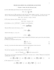
<strong>General</strong> <strong>Relativity</strong>: <strong>Homework</strong> 4 <strong>Solutions</strong><br />
1. Carroll Problem 4.1<br />
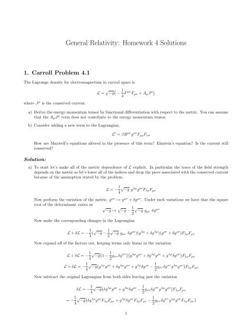
The Lagrange density for electromagnetism in curved space is<br />
where J µ is the conserved current.<br />
L = √ −g ( − 1 4 F µν F µν + A µ J µ)<br />
a) Derive the energy-momentum tensor by functional differentiation with respect to the metric. You can assume<br />
that the A µ J µ term does not contribute to the energy momentum tensor.<br />
b) Consider adding a new term to the Lagrangian,<br />
L ′ = βR µν g ρσ F µρ F νσ<br />
How are Maxwell’s equations altered in the presence <strong>of</strong> this term? Einstein’s equation? Is the current still<br />
conserved?<br />
Solution:<br />
a) To start let’s make all <strong>of</strong> the metric dependence <strong>of</strong> L explicit. In particular the trace <strong>of</strong> the field strength<br />
depends on the metric so let’s lower all <strong>of</strong> the indices and drop the piece associated with the conserved current<br />
because <strong>of</strong> the assumption stated by the problem.<br />
L = − 1 4√ −g g λµ g ρν F λρ F µν<br />
Now perform the variation <strong>of</strong> the metric, g µν ↦→ g µν + δg µν . Under such variations we have that the square<br />
root <strong>of</strong> the determinant varies as<br />
√ √ 1√ −g ↦→ −g − −g gµν δg µν<br />
2<br />
Now make the corresponding changes in the Lagrangian<br />
L + δL = − 1 4 (√ −g − 1 2√ −g gµν δg µν )(g λµ + δg λµ )(g ρν + δg ρν )F λρ F µν<br />
Now expand all <strong>of</strong> the factors out, keeping terms only linear in the variation<br />
L + δL = − 1 √ ( 1 −g 1 −<br />
4 2 g στ δg στ )( g λµ g ρν + δg λµ g ρν + g λµ δg ρν) F λρ F µν<br />
L + δL = − 1 4√ −g<br />
(<br />
g λµ g ρν + δg λµ g ρν + g λµ δg ρν − 1 2 g στ δg στ g λµ g ρν) F λρ F µν<br />
Now subtract the original Lagrangian from both sides leaving just the variation<br />
δL = − 1 4√ −g<br />
(<br />
δg λµ g ρν + g λµ δg ρν − 1 2 g στ δg στ g λµ g ρν) F λρ F µν<br />
= − 1 √ (<br />
−g δg λµ g ρν F λρ F µν + g λµ δg ρν F λρ F µν − 1 4<br />
2 g στ δg στ g λµ g ρν )<br />
F λρ F µν<br />
1
Now take some care in permuting the indices <strong>of</strong> F µν in the fist term, remembering that it is antisymmetric,<br />
so we will flip the indices <strong>of</strong> both factors and raise one <strong>of</strong> them<br />
δL = − 1 √ (<br />
−g δg λµ F ρλ F ρ µ + δg ρν F µ<br />
4<br />
ρF µν − 1 2 g στ δg στ F µν )<br />
F µν<br />
Since there are no free indices we can relabel any paired indices within a given term. In particular we should<br />
look to match all <strong>of</strong> the indices <strong>of</strong> the variation term.<br />
⇒<br />
δL<br />
δg µν = −1 4<br />
δL = − 1 √ (<br />
−g δg µν F ρµ F ρ ν + δg µν F ρ<br />
4<br />
µF ρν − 1 2 g µνδg µν F λρ )<br />
F λρ<br />
√ (<br />
−g Fλµ F λ ν + F λ µF λν − 1 2 g µνF λρ ) 1√ (<br />
F λρ = − −g 2F<br />
λ<br />
4<br />
µ F λν − 1 2 g µνF λρ )<br />
F λρ<br />
So finally we have the energy-momentum tensor<br />
T µν = − 2 √ −g<br />
δL<br />
δg µν = F λ µF λν − 1 4 g µνF λρ F λρ<br />
b) Let’s look at the full Lagrangian (where the field strength tensor has all lower indices) to get an idea <strong>of</strong> how<br />
the resulting equations <strong>of</strong> motion might change<br />
L + L ′ = √ −g ( − 1 4 gλµ g ρν F λρ F µν + A µ J µ + βR µν g ρσ F µρ F νσ<br />
)<br />
To see how this new term affects Maxwell’s equations we should focus on the parts containing the field<br />
strength tensor (see Carroll §1.10). Using the freedom to relabel the indices, we will make it so that the field<br />
strength tensors in each term have matching indices, and then factor that term out<br />
L+L ′ = √ −g ( − 1 4 gλµ g ρν F λρ F µν +A µ J µ +βR λµ g ρν F λρ F µν<br />
)<br />
=<br />
√ −g<br />
(<br />
−<br />
1<br />
4 gλµ g ρν +βR λµ g ρν) F λρ F µν + √ −gA µ J µ<br />
Now to derive Maxwell’s equations (i.e. the equations <strong>of</strong> motion for the field A µ ) we should derive the Euler-<br />
Lagrange equations corresponding to variations <strong>of</strong> A µ and ∇ ν A µ (demanding covariant equations). However<br />
note that the only term dependent upon ∇ ν A µ is the field strength tensor.<br />
δ<br />
δ(∂ σ A τ ) [F δ<br />
λρF µν ] =<br />
δ(∇ σ A τ ) [(∇ λA ρ − ∇ ρ A λ )(∇ µ A ν − ∇ ν A µ )]<br />
= (δ σ λδ τ ρ − δ σ ρ δ τ λ)(∇ µ A ν − ∇ ν A µ ) + (∇ λ A ρ − ∇ ρ A λ )(δ σ µδ τ ν − δ σ ν δ τ µ)<br />
= (δ σ λδ τ ρ − δ σ ρ δ τ λ)F µν + F λρ (δ σ µδ τ ν − δ σ ν δ τ µ)<br />
Therefore the variational derivative <strong>of</strong> the Lagrangian is<br />
δ(L + L ′ )<br />
δ(∂ σ A τ ) = √ −g ( − 1 4 gλµ g ρν + βR λµ g ρν) [(δ σ λδ τ ρ − δ σ ρ δ τ λ)F µν + F λρ (δ σ µδ τ ν − δ σ ν δ τ µ)]<br />
= √ −g ( F τσ + 2β(R σµ g τν − R τµ g σν ) √ (<br />
)F µν = −g F τσ + 2βR µ[τ F σ] )<br />
µ<br />
We can now write out Maxwell’s equation<br />
(<br />
∇ µ F νµ + 2βR λ[ν F µ] )<br />
λ = J<br />
ν<br />
A quick check shows that we recover the usual equation when β goes to zero. Because mixed partial derivatives<br />
commute and the new term is antisymmetric in µ and ν, we see that the current is still conserved locally ,<br />
that is ∂ ν J ν = 0, however because covariant derivatives do not commute, the current is not conserved globally ,<br />
that is ∇ ν J ν ≠ 0.<br />
2
Now we must consider variations <strong>of</strong> the metric to see how this new term affects Einstein’s equation. Let’s<br />
consider the terms that will vary.<br />
L ′ + δL ′ = β( √ −g + δ √ −g)(R µν + δR µν )(g ρσ + δg ρσ )F µρ F νσ<br />
= √ −gβF µρ F νσ (R µν g ρσ + g ρσ δR µν + R µν δg ρσ − 1 2 Rµν g ρσ g λγ δg λγ )<br />
⇒ δL ′ = √ −gβF µρ F νσ (g ρσ δR µν + R µν δg ρσ − 1 2 Rµν g ρσ g λγ δg λγ )<br />
We must now figure out δR µν in terms <strong>of</strong> the variation <strong>of</strong> the metric (note that the argument in Carroll that<br />
this variation disappears, fails in this case because we are not contracting with g µν ). Recall that<br />
R µν = g µα g νγ R λ αλγ<br />
and so the variation is<br />
δR µν = g µα g νγ δR λ αλγ<br />
Now let’s pluck the variation <strong>of</strong> the Riemann tensor and Christ<strong>of</strong>fel symbols from Carroll (eqs. 4.62 and 4.64)<br />
δR λ αλγ = ∇ λ (δΓ λ γα) − ∇ γ (δΓ λ λα)<br />
δΓ λ γα = − 1 2 [g ρα∇ γ (δg ρλ ) + g ργ ∇ α (δg ρλ ) − g ασ g γτ ∇ λ (δg στ )]<br />
Putting this into the expression for the variation <strong>of</strong> the Riemann tensor gives us<br />
δR λ αλγ = − 1 2 [g ργ∇ λ ∇ α (δg ρλ ) − g ασ g γτ ∇ λ ∇ λ (δg στ ) + g ασ ∇ λ ∇ γ (δg σλ ) − ∇ γ ∇ α (g ρλ δg ρλ )]<br />
δR λ αλγ = − 1 2 [∇ λ∇ α (δg λ γ) − ∇ γ ∇ α (δg λ λ) + ∇ λ ∇ γ (δg λ α) − g ασ g γτ ∇ λ ∇ λ (δg στ )]<br />
⇒ δR µν = g µα g νγ δR λ αλγ = − 1 2 [∇ λ∇ µ (δg λν ) − ∇ ν ∇ µ (δg λ λ) + ∇ λ ∇ ν (δg λµ ) − δ µ σδ ν τ ∇ λ ∇ λ (δg στ )]<br />
δR µν = − 1 2 [∇ λ∇ µ (δg λν ) − ∇ ν ∇ µ (δg λ λ) + ∇ λ ∇ ν (δg λµ ) − ∇ λ ∇ λ (δg µν )]<br />
Now just focus on the variation <strong>of</strong> the action due to the variation <strong>of</strong> the Ricci tensor<br />
∫ ∫<br />
√−gβFµρ<br />
δS R = F νσ g ρσ δR µν = − 1 −gβFµρ F νσ g<br />
2√ ρσ [∇ λ ∇ µ (δg λν )−∇ ν ∇ µ (δg λ λ)+∇ λ ∇ ν (δg λµ )−∇ λ ∇ λ (δg µν )]<br />
Now integrate by parts twice, using the fact that the variation and it’s covariant derivative vanish at the<br />
boundary to arrive at<br />
∫<br />
δS R = − 1 √ [<br />
−gβ ∇ µ ∇ λ (F µρ F νσ g ρσ )δg λν −∇ µ ∇ ν (F µρ F νσ g ρσ )δg λ<br />
2<br />
λ+∇ ν ∇ λ (F µρ F νσ g ρσ )δg λµ −∇ λ ∇ λ (F µρ F νσ g ρσ )δg µν]<br />
Now do some relabelling<br />
∫<br />
δS R = − 1 √ [<br />
−gβ ∇ λ ∇ µ (F λρ F νσ g ρσ )−∇ λ ∇ γ (F λρ F γσ g ρσ )g µν +∇ λ ∇ µ (F νρ F λσ g ρσ )−∇ λ ∇ λ (F µρ F νσ g ρσ ) ] δg µν<br />
2<br />
So now the variation <strong>of</strong> the new term is<br />
δL ′ = √ (<br />
−gβ − 1 [<br />
∇ λ ∇ µ (F λρ F νσ g ρσ ) − ∇ λ ∇ γ (F λρ F γσ g ρσ )g µν + ∇ λ ∇ µ (F νρ F λσ g ρσ ) − ∇ λ ∇ λ (F µρ F νσ g ρσ ) ]<br />
2<br />
+F µρ F νσ R ρσ − 1 2 Rλγ g ρσ F λρ F γσ g µν<br />
)<br />
δg µν<br />
3
and Einstein’s equation now reads<br />
(<br />
R µν − 1 2 Rg µν + β − 1 ∇<br />
2[ λ ∇ µ (F λρ F νσ g ρσ ) − ∇ λ ∇ γ (F λρ F γσ g ρσ )g µν + ∇ λ ∇ µ (F νρ F λσ g ρσ )<br />
−∇ λ ∇ λ (F µρ F νσ g ρσ ) ] + F µρ F νσ R ρσ − 1 2 Rλγ g ρσ F λρ F γσ g µν<br />
)<br />
= T µν<br />
where T µν is the energy momentum tensor associated with the electromagnetic field derived in part a.<br />
2.<br />
The point <strong>of</strong> this exercise is to compute the first correction to the Newtonian solution caused by a source that<br />
rotates. In Newtonian gravity, the angular momentum <strong>of</strong> the source does not affect the field: two sources with<br />
identical densities, ρ(x i ), but different angular momenta have the same gravitational field. This is not so in <strong>General</strong><br />
<strong>Relativity</strong>, since all components <strong>of</strong> T µν generate the field. This is an example <strong>of</strong> a post-Newtonian effect.<br />
a) Suppose a spherical body <strong>of</strong> uniform density ρ and radius R rotates rigidly about the x 3 axis with constant<br />
angular velocity ω. Write down the components T 0ν in a Lorentz frame at rest with respect to the center <strong>of</strong><br />
mass <strong>of</strong> the body, assuming ρ, ω, and R are independent <strong>of</strong> time. For each component, work to the lowest<br />
non-vanishing order in ωR.<br />
b) The general solution to the equation ∇ 2 f = g, that vanishes at infinity, is the generalization <strong>of</strong> Φ(r) = −Gm/r,<br />
f(x) = − 1 ∫<br />
4π<br />
g(y)<br />
|x − y| d3 y<br />
Use this to solve Einstein’s Equation, keeping only terms linear in the perturbation, for the components <strong>of</strong><br />
the trace-reversed perturbation h 00 and h 0i , where h µν = h µν − 1 2 ηµν h, for the source described in part (a).<br />
Obtain solutions only outside the body and only to the lowest non-vanishing order in r −1 , where r is the<br />
distance from the center <strong>of</strong> the body. Express the result for h 0i in terms <strong>of</strong> ω. Find the metric tensor within<br />
this approximation and transform it to spherical coordinates.<br />
c) Since the metric is independent <strong>of</strong> t and the azimuthal angle, φ, particles orbiting this body will have constant<br />
p 0 and p φ along their trajectories. Consider a particle <strong>of</strong> non-zero rest mass in a circular orbit <strong>of</strong> radius r in<br />
the equitorial plane. To lowest order in ω, calculate the difference between its orbital period when it’s orbiting<br />
with the direction <strong>of</strong> the body’s rotation (prograde) and when it’s orbiting against the direction <strong>of</strong> the body’s<br />
rotation (retrograde). (Define the period to be the coordinate time taken for one orbit <strong>of</strong> ∆φ = 2π).<br />
Solution:<br />
a) Given that we are doing a small perturbation to the Newtonian solution, we should assume that the rotation<br />
<strong>of</strong> the body is non-relativistic (ωR
1<br />
from this we can determine the factor γ = √ , where we will use the unperturbed metric η<br />
dx µ dx ν<br />
µν to<br />
gµν<br />
dt dt<br />
calculate.<br />
1<br />
⇒ γ =<br />
1 − ω 2 r 2 ≈ 1 + ω2 r 2<br />
Now we can write out the 4-velocity<br />
U µ = dxµ<br />
dτ<br />
= γ dxµ<br />
dt<br />
= γ(1, −ωr sin ωt sin θ, ωr cos ωt sin θ, 0)<br />
which to first order in ωR is just dxµ<br />
dt<br />
(i.e. γ = 1). Now we can calculate the components T 0ν for the<br />
energy-momentum tensor (for r = √ x 2 + y 2 + z 2 ≤ R):<br />
T 00 = ρU 0 U 0 = ρ<br />
T 01 = ρU 0 U 1 = −ρωy<br />
T 02 = ρU 0 U 2 = ρωx<br />
T 03 = ρU 0 U 3 = 0<br />
b) We will now use Einstein’s equation (with upper indices) to solve for the perturbation to the metric.<br />
R µν − 1 2 Rgµν = 8πGT µν<br />
where<br />
g µν = η µν − h µν<br />
We will be dealing with the case where |h µν |
equations, we are free to choose our coordinates. There are four coordinates, so we can equivalently enforce<br />
four conditions on the solution to our metric. Before we decide what conditions to impose, let’s write the<br />
Einstein tensor in terms <strong>of</strong> the trace-reversed perturbation h µν = h µν − 1 2 hηµν<br />
G µν = 1 (<br />
∂ µ ∂ λ (h νλ + 1 2<br />
2 hηνλ )+∂ ν ∂ λ (h µλ + 1 2 hηµλ )−∂ λ ∂ λ (h µν + 1 2 hηµν )−∂ µ ∂ ν h+η µν ∂ λ ∂ λ h−η µν ∂ λ ∂ ρ (h λρ + 1 2 hηλρ ) )<br />
which simplifies to<br />
G µν = 1 (<br />
∂ µ ∂ λ h νλ + ∂ ν ∂ λ h µλ − η µν ∂ λ ∂ ρ h λρ − ∂ λ ∂ λ h µν )<br />
2<br />
Now we can decide what conditions we would like to put on the perturbation terms in order to simplify the<br />
calculations. Noting that the four-divergence <strong>of</strong> the perturbation comes up in three <strong>of</strong> the four terms, if we<br />
enforced the four equations<br />
∂ λ h µλ = 0<br />
then, after neglecting the time derivatives, we are led to the tidy expression<br />
G µν = − 1 2 ∇2 h µν<br />
and now Einstein’s equation reads<br />
− 1 2 ∇2 h µν = 8πGT µν<br />
The only non-zero terms in the energy-momentum tensor are those with at least one time component. Therefore<br />
we can set h ij = 0 for i, j = 1, 2, 3.<br />
Consider the first equation<br />
Let’s use the general form <strong>of</strong> the solution to solve<br />
∫<br />
h 00 (r) = 4Gρ<br />
∇ 2 h 00 = −16πGρ<br />
1<br />
|r − r ′ | d3 r ′ ≈ 4Gρ 1 ∫<br />
r<br />
d 3 r ′ = 16πGρR3<br />
3r<br />
= 4GM<br />
r<br />
1<br />
where we have just taken the first order term <strong>of</strong> the Taylor expansion<br />
|r−r ′ | = 1 r′·ˆr<br />
r<br />
(1 +<br />
r<br />
+ ...) for r >> r ′ .<br />
Now consider<br />
∇ 2 h 01 = −16πGρωy<br />
the solution to which is<br />
∫<br />
h 01 y ′ d 3 r ′<br />
(r, θ, φ) = 4Gρω<br />
|r − r ′ |<br />
1<br />
where the integral is taken over the source matter. Now expand<br />
|r−r ′ |<br />
to the first two orders, this will be<br />
necessary because we will see that the first order term will be zero.<br />
∫<br />
h 01 (r, θ, φ) = 4Gρω<br />
( 1 r + r′ · ˆr<br />
r 2 )y′ d 3 r ′ = 4Gρω<br />
∫ ( 1<br />
r y′ + r′ · ˆr<br />
r 2 y′) d 3 r ′<br />
The source matter has a spherical distribution, and as such the region <strong>of</strong> integration is symmetric under sign<br />
changes <strong>of</strong> the coordinates. We may then see that the first term in the integral, being odd in y ′ , will yield no<br />
contribution.<br />
h 01 (r, θ, φ) = 4Gρω 1 ∫<br />
r 2 (r ′ · ˆr)y ′ d 3 r ′ = 4Gρω 1 ∫<br />
r 2 (x ′ cos φ sin θ + y ′ sin φ sin θ + z ′ cos θ)y ′ d 3 r ′<br />
h 01 (r, θ, φ) = 4Gρω sin θ sin φ < y2 ><br />
r 2<br />
6
where we have used the notation < y 2 >= ∫ y ′2 d 3 y ′ , to denote the average <strong>of</strong> the square <strong>of</strong> the y-coordinate<br />
on the sphere and that ˆr = (cos φ sin θ, sin φ sin θ, cos θ). We have also used symmetry to deduce that the x ′ y ′<br />
and z ′ y ′ terms in the integrand will not contribute. Similarly we deduce<br />
We also know that because T 03 vanishes, h 03 = 0.<br />
h 02 (r, θ, φ) = − 4Gρω sin θ cos φ < x2 ><br />
r 2<br />
Now let’s translate back to the metric perturbations, which gives us the following equations<br />
h µµ = h µµ − h<br />
h 01 = h 01<br />
h 02 = h 02<br />
h 03 = h 03<br />
h = −h 00 + h 11 + h 22 + h 33<br />
We can see readily that<br />
h 01 = 4Gρω sin θ sin φ < y2 ><br />
r 2<br />
h 02 = − 4Gρω sin θ cos φ < x2 ><br />
r 2<br />
h 03 = 0<br />
Because h ii = 0 for i = 1, 2, 3 we have that h ii = 1 2 h (which implies all hµµ are equal) so we can write the<br />
trace entirely in terms <strong>of</strong> h 00 h = 2h 00<br />
and we have h 00 = h 00 − 1 2 (2h00 ) which implies<br />
h µµ = 1 2 h00 = 2GM<br />
r<br />
Now let’s transform from Cartesian to spherical coordinates using the transformation law for (0, 2)-tensors.<br />
h 0r = ∂x<br />
∂r h 01 + ∂y<br />
∂r h 02 = (cos φ sin θ) ( −4Gρω sin θ sin φ < y 2 ><br />
r 2 )<br />
+ (sin φ sin θ)<br />
(4Gρω sin θ cos φ < x 2 ><br />
r 2 )<br />
= 0<br />
where we’ve used that by the spherical symmetry <strong>of</strong> the source distribution < x 2 >=< y 2 >.<br />
h 0φ = ∂x<br />
∂φ h 01 + ∂y<br />
∂φ h 02<br />
h 0φ = (−r sin φ sin θ) ( −4Gρω sin θ sin φ < y 2 > ) (4Gρω sin θ cos φ < x 2 > )<br />
+ (r cos φ sin θ)<br />
r 2 r 2<br />
h 0φ = 4Gρω sin2 θ(< x 2 > + < y 2 >)<br />
r<br />
While they are equal we have kept the distinction between < x 2 > and < y 2 > so that we may make an<br />
observation. In particular the combination ρ(< x 2 > + < y 2 >) = ∫ ρ(x ′2 + y ′2 )d 3 r ′ is equal to the moment<br />
<strong>of</strong> inertia about the z-axis <strong>of</strong> the sphere (for a uniform sphere this is I = 2 5 MR2 = 8π 5 ρR5 ). We may then<br />
rewrite this component as<br />
h 0φ = 4G sin2 θL<br />
r<br />
where L = Iω is the angular momentum <strong>of</strong> the source matter.<br />
Let’s focus on the remaining non-zero components <strong>of</strong> the metric,<br />
7
h rr = ( ∂x<br />
∂r<br />
) 2h11<br />
+ ( ∂y<br />
∂r<br />
) 2h22<br />
+ ( ∂z ) 2h33<br />
= 8πGρR3<br />
∂r<br />
3r<br />
h φφ = ( ∂x ) 2h11<br />
+ ( ∂y ) 2h22<br />
+ ( ∂z ) 2h33<br />
= 8πGρR3 r sin 2 θ<br />
∂φ ∂φ ∂φ<br />
3<br />
h θθ = ( ∂x) 2h11<br />
+ ( ∂y ) 2h22<br />
+ ( ∂z ) 2h33<br />
= 8πGρR3 r<br />
∂θ ∂θ ∂θ<br />
3<br />
It is easily verified that the remaining <strong>of</strong>f-diagonal terms are zero. Now we can write out the metric as<br />
where Φ = − GM r<br />
ds 2 = −(1 + 2Φ)dt 2 + 4G sin2 θL<br />
(dtdφ + dφdt) + (1 − 2Φ)(dr 2 + r 2 sin 2 θdφ 2 + r 2 dθ 2 )<br />
r<br />
= − 4πGρR3<br />
3r<br />
.<br />
c) A particle in orbit in the equatorial plane will have the trajectory<br />
x µ = (t, r, φ(t), π 2 )<br />
Now consider the r-component <strong>of</strong> the geodesic equation for such trajectories (i.e. constant r and θ = π/2)<br />
d 2 r<br />
dτ 2 + ( dt ) 2 Γr tt + Γ<br />
r<br />
(dφ) 2 (<br />
dτ φφ + 2Γ<br />
r dt dφ) dτ<br />
φt = 0<br />
dτ dτ<br />
⇒ Γ r ( dt ) 2<br />
tt + Γ<br />
r<br />
(dφ) 2 (<br />
dτ φφ + 2Γ<br />
r dt dφ) dτ<br />
φt = 0<br />
dτ dτ<br />
Because the metric is t and φ independent we see that<br />
Γ r tt = − 1 2 grr ∂ r g tt<br />
Γ r φφ = − 1 2 grr ∂ r g φφ<br />
Γ r φt = − 1 2 grr ∂ r g φt<br />
If we assume that the body is orbiting slowly (so that we may assume t ≈ τ) the geodesic equation may then<br />
be written as<br />
(dφ) 2 (dφ) ∂ r g tt + ∂ r g φφ + 2∂r g φt = 0<br />
dt<br />
dt<br />
Plugging in the metric components we have<br />
−∂ r (1 − 2GM ) + ∂ r (r 2 + 2GMr) ( dφ) 2<br />
+ 2∂r ( 4GL<br />
r<br />
dt<br />
r<br />
)( dφ) = 0<br />
dt<br />
− 2GM<br />
r 2 + 2(r + GM) ( dφ) 2 8GL(dφ) − = 0<br />
dt r 2 dt<br />
which we can rewrite as<br />
r 2 (1 +<br />
r<br />
GM )( dφ) 2 4L(dφ) − − 1 = 0<br />
dt M dt<br />
Recognizing this equation as a quadratic, we solve for dφ<br />
dt<br />
4L<br />
dφ<br />
dt =<br />
M ± √<br />
16L 2<br />
M 2 + 4r 2 (1 + r<br />
2r 2 (1 +<br />
Now we may calculate the difference in the orbital period<br />
∆T = 2π | dφ<br />
dt − | − | dφ<br />
dt + |<br />
| dφ dφ<br />
dt + dt − |<br />
r<br />
GM )<br />
GM )<br />
( 4L )(<br />
M<br />
= 2π<br />
r 2 (1 +<br />
r<br />
GM )<br />
∆T = 8πL<br />
M<br />
= 16π<br />
5 R2 ω<br />
r 2( 1 +<br />
r ) )<br />
GM<br />
Note that when L → 0 the difference in orbital period is zero, as we should expect.<br />
8
3.<br />
In the presence <strong>of</strong> a cosmological constant Λ, Einstein’s equation is<br />
R µν − 1 2 Rg µν + Λg µν = 8πGT µν<br />
a) Calculate the gravitational potential Φ in the Newtonian limit outside a spherically symmetric point source<br />
with ρ = Mδ 3 (r).<br />
b) A good description <strong>of</strong> the gravitational forces in our solar system is given by Newton’s potential, Φ =<br />
−GM ⊙ /r, where M ⊙ is the mass <strong>of</strong> the sun. Use this fact to determine an upper limit for the vacuum energy<br />
density ρ Λ = Λ/8πG, given that the radius <strong>of</strong> Pluto’s orbit is r P luto ≈ 6 × 10 12 m. Express your answer in<br />
GeV 4 .<br />
Solution:<br />
a) Follow the steps in Carroll §4.2 to derive Poisson’s equation from Einstein’s equation in the Newtonian limit.<br />
∇ 2 Φ = 4πGρ<br />
Now set ρ = Mδ 3 (r) − ρ Λ . The spherical symmetry <strong>of</strong> the distribution requires that the potential should only<br />
depend on r, the distance from the point source, that is we should look for a solution <strong>of</strong> the form Φ(r).<br />
Poisson’s equation now reads<br />
∇ 2 Φ = 4πG(Mδ 3 (r) − ρ Λ (r))<br />
Now integrate both sides over the volume <strong>of</strong> a sphere <strong>of</strong> radius r ′<br />
∫<br />
∫<br />
∇ 2 Φ dV = 4πG (Mδ 3 (r) − ρ Λ (r))dV<br />
First look at the right hand side and note that we can apply Stokes’ theorem<br />
∫<br />
∫<br />
∫<br />
∇ 2 Φ dV = ∇ · (∇Φ)dV = (∇Φ) · dS<br />
where the integral is now over the surface <strong>of</strong> the sphere. Due to spherical symmetry ∇Φ must point in the ˆr<br />
direction and be constant on the surface <strong>of</strong> the sphere, therefore the integral now becomes<br />
∫<br />
∇ 2 Φ dV = 4πr ′2 |∇Φ|<br />
Now we deal with the right hand side:<br />
∫<br />
4πG<br />
(Mδ 3 (r) − ρ Λ (r))dV = 4πGM − 16π2 G<br />
ρ Λ r ′3<br />
3<br />
Putting the two together we have:<br />
∇Φ(r ′ ) = ( GM<br />
r ′2 − 4π 3 Gρ Λr ′)ˆr<br />
Now to solve for Φ we just integrate ∇Φ from the edge <strong>of</strong> the universe (let’s call it ∞) to r.<br />
Φ(r) = Φ(∞) +<br />
∫ r<br />
∞<br />
∇Φ · dˆr = Φ(∞) +<br />
∫ r<br />
∞<br />
( GM<br />
r ′2 − 4π 3 Gρ Λr ′ )dr ′ = − GM r<br />
− 4π 3 Gρ Λr 2<br />
where we’ve cancelled out the potential at infinity with the evaluation <strong>of</strong> the anti-derivative at the edge <strong>of</strong><br />
the universe.<br />
9
) To find an upper bound on the vacuum energy density, we will find what value is necessary to keep Pluto<br />
bound to the solar system. We can write this as the requirement that the negative gradient <strong>of</strong> the potential<br />
(i.e. the acceleration) be negative (so that the acceleration is towards the center <strong>of</strong> the solar system).<br />
Isolating the vacuum energy density we arrive at<br />
−∇Φ(r P luto ) = − GM ⊙<br />
rP 2 + 4π<br />
luto<br />
3 Gρ Λr P luto < 0<br />
ρ Λ < 3<br />
4π<br />
M ⊙<br />
r 3 P luto<br />
= 3 1.989 × 10 30 kg ( 1GeV )(1.97 × 10 −16 m<br />
4π (6 × 10 12 m) 3 1.78 × 10 −27 kg GeV −1 ) 3<br />
ρ Λ < 9.44 × 10 −30 GeV 4 ≈ 10 −29 GeV 4<br />
10