Applications of the Windowed FFT to Electric Power Quality ...

Application of the Global Positioning System to the Measurement of Overhead Power
Transmission Conductor Sag
C. Mensah-Bonsu U. Fernández G. T. Heydt Y. Hoverson J. Schilleci B. Agrawal
Student Member Student Member Fellow Non-Member Senior Member Fellow
Center for the Advanced Control of Energy and Power Systems
Arizona State University, Tempe, AZ
Entergy
New Orleans, LA
Arizona Public Service
Phoenix, AZ
Abstract This paper describes a method to directly measure
the physical sag of overhead electric power transmission
conductors. The method used relies on the Global
Positioning System (GPS) used in the differential mode.
The direct measurement of sag is a main advantage of the
concept. The digital signal processing required is described
in detail in a four level configuration. Typical accuracy,
response time, problems, strengths and weaknesses
of the method are also described.
Keywords: Global Positioning System; overhead conductors;
sag; dynamic line rating; transmission engineering;
Open Access Same Time Information System(OASIS).
1. Overhead conductor ratings
Under deregulation of the power industry in the United
States, electric utilities are under pressure to make optimum
use of their existing facilities of which the overhead
transmission system is usually a principal component.
Overhead conductors form the backbone of power transmission
systems. The ratings of circuits are critical to system
capability. Real time conductor rating holds promise
for the maximization of system transfer capability.
The transmission capacity of overhead conductors depends
on the ambient temperature, wind speed, wind direction,
incident solar radiation, limiting physical conductor
characteristics, and conductor configuration / geometry.
The conductor load capacity is computed statically or dynamically.
In the static case, a worst case weather condition
is assumed while in the dynamic case the actual
weather condition is taken into account. In either case, the
conductor load must produce a conductor temperature so
that there is no loss of strength by annealing or creep. One
must operate the circuit so that the mandated clearances are
not violated. Experience in some utilities shows that the
clearance of an overhead conductor is a key factor limiting
its thermal capacity especially in regions of high intercon-
nection. An ultimate measure of the conductor rating is the
physical sag of the conductor and the continuous monitoring
of the conductor clearance may improve system operation.
This paper considers the use of a GPS based measurement
system for overhead conductor sag – based on
tests using a laboratory breadboarded prototype.
Traditionally, conductor sag has been considered by
indirect measurements. Recently commercialized techniques
include the physical measurement of conductor surface
temperature using an instrument mounted directly on
the line, and a second instrument that measures conductor
tension at the insulator supports. These measured parameters
can be used to estimate conductor sag. The pertinence
of conductor sag to circuit operation relates to the calculation
of a dynamic thermal rating of the line, considering
the ambient conditions and present operating regime [1-5].
In a deregulated electric utility environment, transmission
circuit ratings assume renewed importance because some
companies are marketing transmission access. A widely
used system for transmission capacity sales is known as
OASIS. To be able to rapidly and accurately determine the
dynamic transmission rating of a circuit has obvious pecuniary
value in OASIS.
2. The Global Positioning System
Based on a constellation of 24 satellites, the Navigation
Satellite Timing and Ranging (NAVSTAR) GPS was developed,
launched and maintained by the United States
government as a worldwide navigation and positioning
resource for both military (i.e. precise positioning service)
and civilian (i.e. standard positioning service) applications.
The method relies on accurate time-pulsed radio signals in
the order of nanoseconds from high altitude Earth orbiting
satellites of about 11,000 nautical miles, with the satellites
acting as precise reference points. These signals are
transmitted on two carrier frequencies known as the L1 and
L2 frequencies. The L1 carrier is 1.5754 GHz and carries
a pseudorandom code (PRC) and the status message of the
satellites. There exist two pseudorandom codes; the
coarse acquisition (C/A) and the precise (P) codes. The L2
carrier is 1.2276 GHz and is used for the more precise military
PRC. The signals from four or more satellites are received
by a specially designed GPS receiver, and the following
simultaneous equations are solved,
2
2
2
2
( X
sk
− X
rj
) + ( Ysk
− Yrj
) + ( Z
sk
− Zrj)
= ( Rk
− dT )
k = 1, 2, …, n n ≥ 4 (1)
where (X sk , Y sk , Z sk ) represents the kth satellite position, (X rj
Y r , Z rj ) denotes the unknown jth receiver position, R k denotes
the range to the kth satellite and dT is the unknown

eceiver clock bias converted to distance. This gives the
longitude and latitude of the receiver (i.e., effectively x and
y), the altitude of the receiver (effectively z), and the time
that the measurement was made, t. Interestingly, the GPS
transmission is made at low power level (the signal
strength at the point of reception is about –90 to –120
dBm); at this power level, the signal to noise ratio is very
low at the surface of the Earth. The attenuation of the
noise is accomplished by averaging the received signal:
the noise is averaged and a distinctively coded signal appears
as an output. The averaging process as well as the
solution of Equation (1) is the main time limiting process
that determine how often a GPS measurement can be
made.
Perhaps the most often asked question about GPS technology
relates to its accuracy. The ultimate accuracy of
position measurements made using the GPS depend on a
variety of factors (e.g., the type of measurement made, x, y,
or z; ionospheric and tropospheric conditions; government
inserted error effected as a security measure; number of
satellites in view; receiver equipment used; digital signal
processing of the received signal; surface features; reflection
of signals; and other factors). Table (1) summarizes
some of these interacting factors and the approximate error.
In Table (1), a differential mode of measurement is
also shown, and this is discussed later. The greatest source
of error is the intentional insertion of error through a subsystem
known as Selective Availability (SA): this error is
inserted by the government as a security measure. Authorized
non-civilian users of a special high accuracy mode of
operation have a special mechanism to decode the SA and
eliminate the intentional error.
Table (1) Approximate GPS position measurement error
(total) contributing factors and estimates
Approximate error (m)
Error contributing factor Standard DGPS
GPS
Selective availability (SA) 30.0 0.0
Ionospheric variation 5.0 0.4
Inaccurate orbital path 2.5 0.0
Satellite clock 1.5 0
Multipath signal error 0.6 0.6
Tropospheric variation 0.5 0.2
Receiver noise 0.3 0.3
The differential GPS (DGPS) mode is generally used in
order to decrease the SA error. This mode consists of the
use of two GPS receivers, the base and the rover. The actual
position of the base is known (e.g., by precise surveying)
and compared to the readings received at the same
base point. With the estimated error, the readings obtained
at the rover can be compensated by simple subtraction.
The value of the DGPS technique is a marked increase in
instrument accuracy with little degradation of time requirement.
The main drawback of the DGPS technique is
the requirement of a second GPS receiver and corresponding
communication equipment between the base and rover
instruments. Also, if the rover and base instruments are
widely separated, the solution accuracy will degrade. The
term direct DGPS is used to refer to a GPS configuration
in which the position and time measurements are available
at the rover station. The term inverse DGPS refers to a
DGPS instrument in which the results are available at the
base station. Table (2) shows typical position accuracy of
GPS and DGPS [7 – 9].
Table (2) Typical position accuracy of GPS in (m)
Standard GPS Differential GPS
Horizontal 50 1.3
Vertical 78 2.0
Three dimensional 93 2.8
3. GPS Measurement of overhead conductor sag
Figure (1) shows a proposed basic configuration of a
DGPS method to measure overhead transmission conductor
position and hence, sag. Inverse DGPS technology is
used. Normally only one phase of a circuit would be instrumented
in a critical span. From the base station, hardwire
is used to bring position data to power system operators.
Alternately, the base station may be at the operations
center itself. There is a considerable data processing burden
in the implementation of the DGPS: this is needed to
attenuate noise and enhance accuracy. This burden is calculable
in real time using serial on-line processing. The
main time resolution limitations of the instrument are the
calculation of the (x, y, z, t) from the GPS signal and bad
data rejection described in the next section.
4. Data processing from the GPS
The accuracy of GPS measurements depends heavily on
the configuration of the receiver(s) (e.g., standard GPS or
differential), parameters that influence error in measurements,
the number and position of the satellites in view,
and the digital signal processing of the GPS measurements.
The fundamental required data processing is the solution of
the time-distance linear equations,
distance = (velocity) (time),
for the four or more GPS measurements. The form of
these equations is shown in Equation (1). These equations
are usually solved recursively using a previously solved
case as an initialization. This is shown in Figure (2) as the
SATELLITE
BASE
PSEUDORANDOM
CODE
ROVER
Fig. (1) Basic DGPS configuration for conductor sag
measurement
first level of required digital processing. In the case of the
application of DGPS measurements, the application of the
correction signal from a base station receiver is also fun-
SAG

damental. This is shown in Figure (2) as a second level
signal processing. The first and second levels of processing
are done entirely by the GPS engine. The central focus
of interest in the measurement of overhead transmission
conductor sag is in the measurement of altitude, that is z(t).
Level
1 Solution of
timedistance
equations
2 Differential
GPS corrections
3 Bad data
rejection
Z Y X
Solution of
timedistance
equations
Differential
GPS corrections
Bad data
rejection
Solution of
timedistance
equations
Differential
GPS corrections
Bad data
rejection
taken for a set of known positions. The results depicted in
Figure (3) were obtained experimentally using a 12 channel
DGPS receiver at a surveyed position near Phoenix, AZ
at about 359 m above mean sea level taking readings at the
rate of one per second.
Cumulative distribution (%)
Bad data rejected (— )
Raw data (- - -)
4 Tuned filter estimator
Estimate of
Z
Fig. (2) Depiction of four levels of digital signal processing
required for GPS measurements
In level 3 of the data processing, bad data rejection is
used. Bad data result from a variety of causes – some not
fully understood. The momentary loss of some satellites
from view will negatively impact the measurement accuracy.
Also, momentary interference and signal reflections
may degrade accuracy. In addition, the ambient noise impacts
solution accuracy. Other error mechanisms may
also create single datum values that are erroneous.
Identification of bad data is accomplished through the
use of the identification of a measurement which differs
from the mean value (of x, y, or z as appropriate) by greater
than preset tolerance values kσ x , kσ y , kσ z respectively where
the σ values denote the sample standard deviation values of
x, y, and z as measured in a moving window of width T.
The bad datum is replaced with the window mean. Parameter
k is chosen to obtain the proper rejection rate, and
the window width T is chosen shorter than the expected
duration of residence of the conductor in a given position.
Typical values for the present application are k = ±1.0 and
T = 30 s. Considerations in the selection of these parameters
are: expected wind conditions and movement of the
conductor, operators’ requirements of real time values;
and accuracy of the readings. It should be pointed out that
choosing a large T implies the introduction of certain delay,
since the readings of the previous positions may be
still in the window. On the other hand, a very short window
width will produce no rejection.
The effect of the bad data rejection can be observed in
Figure (3), which shows the cumulative distribution of the
absolute value of the error computed from measurements
Absolute value of error (m)
Fig. (3) Effect of bad data rejection
A fourth level of digital signal processing is depicted in
Figure (2). Note that the measurements are made at approximately
0.9 s intervals, and the measured data is available
at discrete values of time. For this reason, it is convenient
to refer to the measured set of data as x(k), y(k),
z(k). The time measurement is not used in this application.
Field trials of a prototype instrument indicate that errors in
x and y often occur simultaneously with errors in z. This
suggests that measured x and y could provide additional
information for corrections in z. In this fourth level of signal
processing, two different techniques have been tested:
a least squares estimator (LSE) and an artificial neural
network estimator (ANNE). Both are separately used as
tuned filter estimators that are trained (tuned) using a
known data set. Surveyed data are used to provide a set of
[x k , y k , z k ] data which are used to select parameters of the
estimators such that the error in the known set is minimized.
For testing purposes, the data set allows the comparison
of estimated x, y, z to known values thereby providing
an estimate of the instrument accuracy.
In trying to capture the nonlinear behavior of the error,
the LSE adopted is formulated as,
)
2 2 2
z( n) = Ax( n) + By( n) + Cz( n) + Dx ( n) + Ey ( n) + Fz ( n)
where x(n), y(n), z(n) are the sampled readings at certain
time that produce the corresponding vertical measurement
estimation z ) ( n)
. Using the set of measurements x(n), y(n),
z(n) taken for a set of known altitude z o and replacing
z ) ( with z o the above equation can be expressed in matrix
form as,
Ζ Known = ΧΘ
where Θ = [ A B C D E F] T . The parameters [ A, B, C, D,
E, F ] are computed using simple state estimation (i.e.,

least squares parameter estimation). One formulation involves
the Moore-Penrose pseudoinverse of the matrix X
[10].
The ANNE is implemented using a time lag feed forward
network [11]. In this configuration, contrary to the
LSE, p previous readings of x, y and z are used to estimate
z. A two-weighted layer network is used, consisting of h
neurons in the hidden layer and one output layer. A sigmoid
function, specifically the logistic function [11] is
employed as the activation function of the hidden neurons,
while the output neuron employs a linear function. The
optimum values of p and h are determined in the tuning
process. A schematic of the network is shown in Figure
(4).
x(n)
.
.
x(n-p)
y(n)
.
.
y(n-p)
z(n)
.
.
z(n-p)
Input
layer
.
.
.
.
Hidden
layer
Output
neuron
)
z (n)
Fig. (4) ANN parameter estimator to correct z(n) data
from a DGPS measurement
Some results of field testing and the details of the
signal processing techniques described here are shown in
the Appendix. Note that through the use of a least squares
estimator, accuracy within 21.5 cm was obtained 70% of
the time, and using an artificial neural network estimator,
an accuracy of at least 19.6 cm is obtained for 70% of the
time (see Table (A1)).
5. Power supply and communications link
For a practical sag measurement instrument, in addition
to the digital signal processing outlined above, there is the
matter of instrument power supply and the communication
link between the base and rover units. Based on a popular
commercial GPS receiver, the power supply requirements
for the base and rover instruments are shown in Table (3).
The power requirements at the base station are derived
from conventional sources. At the rover, power must be
derived from the overhead conductor itself. This concept
has been commercialized in many applications, and laboratory
tests revealed that the technology is easily implemented.
Figure (5) shows one configuration based on a
current transformer (CT) design. Experience shows that
voltage regulation of the GPS receiver supplies is essential.
Communication between the rover and base station is accomplished
using standard digital communications technologies.
A typical communication link consists of ‘onoff’
amplitude modulation for the communication channel,
implemented in the Industrial Scientific and Medical (ISM)
band, 902 - 928 MHz. The design tested in the laboratory
is effectively a serial port connection via radio. Figure (6)
shows a possible configuration. The frequency source in
this design is derived from a voltage controlled oscillator
(VCO) which is held at the proper frequency by a phase
locked loop circuit. The ultimate frequency source is a
quartz crystal (XTAL).
Unit
Rover
Base
Table (3) Instrument power requirements (typical)
Typical power requirements
Component
(DC)
V I P
(volts) (amps) (watts)
GPS receiver 12 2 24
Digital (serial) data transmitter
12 2 24
Digital (serial) data receiver 12 0.2 2.4
GPS receiver 12 2 24
Digital (serial) data transmitter
12 5 60
Digital (serial) data receiver 12 0.2 2.4
CURRENT
CT
PHASE
CONDUCTOR
VOLTAGE
REGULATOR
12 VDC
Fig. (5) Power supply for the rover unit: a magnetic ring
is clamped around the conductor to be instrumented.
ANT AND
LOW NOISE AMPL
GPS
RCVR
PHASE
LOCKED
LOOP
XTAL
SERIAL
PORT
SHIFT
REGISTER
CLOCK
AMPL
MODULATOR
DIFF
AMP FILTER VCO
(a) GPS receiver / rover transmitter
LOW
NOISE
AMP
PHASE
LOCKED
LOOP
XTAL
MIXER
VCO
FILTER
FILTER
AMP
SERIAL
PORT
GPS
SOFTWARE
(b) Base station receiver
Fig. (6) Communication between the rover and base stations
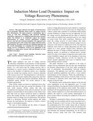
An important issue in the present application is the performance
of the communication link in a high voltage environment
(and, perhaps more serious, the 1.5 GHz band
reception of the GPS signal at the rover). Experiments

have been done to determine the difficulties in these areas
and the main conclusion is that corona creates potentially
intolerable conditions for radio reception in the 930 MHz
and 1.5 GHz bands. There may also be some degree of
‘saturation’ in the receiver front end first stages, but the
use of low noise amplifiers, standard in ISM and GPS
technologies, seems to be adequate. It is important that the
radio receivers at the rover be far from any corona. The
receiver should be ‘shielded’ by instrument packaging that
is smooth and corona free.
6. Dynamic thermal line ratings
As previously discussed, sag information is valuable in
order to determine dynamic thermal rating of overhead
conductors. In present dynamic thermal rating methods,
the sag information is an output, but in this new approach,
the sag information is an input, consequently the rating
computation method must be reviewed. Although it is
beyond the scope of this paper, a tentative method is outlined:
Figure (7) summarizes a procedure to utilize sag
information and translate it to conductor rating.
IEEE Std. 738-1993 to
compute new possible
loading
Sag Reading
Actual conductor
temperature
computation
Actual weather effect
from heat balance
equation
Evaluation of weather
effect to obtain a
confidence index
Fig. (7) Computation of dynamic thermal rating based on
sag information
For specified values of conductor physical characteristics,
i.e., weight per unit of length, modulus of elasticity
and linear coefficient of expansion, and for given installation
conditions of the conductor, the new conductor temperature
can be computed [12]. With the knowledge of the
conductor temperature and current, the net weather influence
in the heat balance equation [2] can be evaluated,
dTc
2
qs
− qc
− qr
= mC p + I R( Tc
) (3)
dt
where q s, q c , q r , mC p , I, R, and T c represent the solar heat
gain, convection heat loss, radiated heat loss, total heat
capacity, conductor current, conductor resistance, and the
conductor temperature respectively. The variations in the
terms of the left side of Equation (3) could be computed
for known variation of the conductor temperature using the
equations and tables suggested in [2]. Using the estimated
initial net weather effect, and with the ability to compute
changes in it, Equation (3) could be again solved for a step
increase in current. Computation in this way, the maximum
current increase that corresponds to the maximum
allowable temperature is found. It should be pointed out
that the variation in the net weather effect is assumed to be
caused only by an increase in the conductor temperature
and not in weather conditions.
Using continuous monitoring of the current and the
conductor temperature (via sag information), the net
weather effect (q s − q c − q r ) can be computed. A highly
variable weather condition implies that the maximum current
computed may not be reliable. On the other hand, if
the net weather is static, confidence is higher. For this reason
a confidence index, based on the variance of the net
weather effect for different time windows is suggested.
Real time measurements of conductor sag have the potential
of being accurately converted to real time, dynamic
line ratings; these dynamic ratings are then useable in
connection with systems studies to determine the maximum
transmission capacity of circuits. The OASIS system
is, in effect, a market for this transmission capacity, and it
is possible that accurate, on-line, dynamic line ratings may
have considerable value.
7. Conclusions
The main conclusion of this study is that DGPS technology
is feasible for the direct instrumentation of overhead
power line conductor sag measurement. The accuracy
of such an instrument is in the range of 19.6 cm 70%
of the time. The method utilizes two GPS receivers, one as
a base station which must be at an accurately surveyed
location. The instrument can be designed such that the
rover receiver operating power is taken from the line. Care
must be taken in the design of the instrument package because
of the potential of interference from corona. The
main digital signal processing needed to obtain accurate z
measurements are bad data rejection, least squares parameter
estimation, or artificial neural network filtering.
Although the subject of dynamic line ratings is not considered
in this paper, it is believed that real time sag measurement
can be translated into real time, dynamic circuit
ratings, and this is expected to have value in the sale of
transmission capacity.
Acknowledgements
The authors acknowledge the assistance of colleagues
at Entergy and the Arizona Public Service Company.
Professors E. Burns, R. Farmer and G. Karady of
ASU and D. Selin of APS are gratefully acknowledged.
Alex Hunt of ASU designed the DGPS receiver circuit, and
several students assisted in the power supply and communications
link designs. John Wells of the United States
Navy is acknowledged for power supply design. The generous
help of R. Faulkner and A. Carbognin and the loan of
GPS receivers from NovAtel Inc., Calgary, were critical to
the work reported. The work was done under the auspices
of the Center for the Advanced Control of Energy and
Power Systems.

References
[1] G. Ramon, IEEE Task Force Chairman: “Dynamic thermal line
rating summary and status of the state-of-the-art technology,” IEEE
Transactions on Power Delivery, v. PWRD-2, No. 3, July 1987, pp.
851-856.
[2] IEEE Std. 738-1993, IEEE Standard for Calculating the Current-
Temperature Relationship of Bare Overhead Conductors, New York,
1993.
[3] T. Seppa, “Accurate ampacity determination: temperature-sag
model for operational real time ratings,” IEEE Transactions on Power
Delivery, v. 10, No. 3, July 1995, pp. 1460-1466
[4] U. Fernández, C. Mensah-Bonsu, J. Wells, G. Heydt, “Calculation
of the maximum steady state transmission capacity of a system,”
Proceedings of the 30th North American Power Symposium, Cleveland,
Ohio, October 19-20, 1998, pp. 300-305.
[5] D. Douglas, A. Edris, “Real-time monitoring and dynamic thermal
rating of power transmission circuits,” Transactions on Power
Delivery, v. 11, No. 3, July 1996, pp. 1407-1415
[6] B. J. Cory, P. F. Gale, "Satellites for power system applications,"
IEE Power Engineering Journal, v. 7 No. 5, October 1993.
[7] J. Hurn, Differential GPS Explained, Trimble Navigation Ltd.,
Sunnyvale, CA 1993.
[8] E. Kaplan, Understanding GPS: Principles and Applications,
1996.
[9] T. Gray, NAVSTAR GPS and DGPS, CSI Inc., 1997.
[10] G. Heydt, Computer Analysis Methods for Power Systems,
Stars in a Circle Publications, Scottsdale, AZ, 1998.
[11] S. Haykin, Neural Networks: A Comprehensive Foundation, 2 nd
Edition, Prentice Hall, New York, NY, 1999.
[12] D. G. Fink, H. W. Beaty (Editors), Standard Handbook for Electrical
Engineers, 13 th Edition, McGraw-Hill, 1993.
Appendix
Signal processing results
In order to test the above described signal processing
procedures, a series of tests were done. One exemplar test
is described as taking DGPS readings for ten known elevations
(stations), collocated in longitude and latitude. The
altitude difference between stations varies between 0.10 to
1.0 m. An average of 1800 readings were taken for each
station. From the ten stations, five were used to tune the
estimators and the rest were used to test the performance of
the estimators in the presence of data not previously seen.
The bad data rejection in the third level has been computed
using values of k = 1 and T = 30 s. These have presented a
good performance regarding excessive number of data rejection
and the response time, as explained previously. For
the ANNE, several configurations have been explored regarding
the number of neurons in the hidden layer. Good
results were obtained for h = 4. In all cases, the number of
previous readings used have been p = 9. With the configurations
described the results obtained are summarized in
Figure (A1).
It can be seen that for a 90% confidence the LSE and
ANNE present respectively an accuracy of 41.9 cm and
37.4 cm. For 70% confidence, the respective accuracy are
21.5 cm and 19.6 cm. Table (A1) summarizes the accuracy
obtained with the respective confidence index. In
Table (A1), note that there is an additional 5 cm uncertainty
in the antenna position, and at least 5 cm potential
survey error. It is expected that the inaccuracies tabulated
are conservative. It can be seen that the ANNE presents
slightly better results. However, both estimator present
similar performance.
Cumulative distribution (%)
Absolute value of error (m)
ANNE (— )
LSE (- - -)
Fig. (A1) Cumulative error for LSE and ANNE
Table (A1) Accuracy achieved by LSE and ANNE
Absolute error (cm)
Confidence Raw Bad data
LSE ANNE
Index (%) data rejected
90 264.4 78.5 41.9 37.4
80 201.8 58.9 30.1 24.5
70 161.1 45.5 21.5 19.6
60 128.9 34.9 15.4 14.6
50 100.6 27.9 11.8 11.4
Biographies
Chris Mensah-Bonsu was born in Kumasi, Ghana. He received
Masters degrees in Control Systems and Electric Power Engineering
from Cleveland State University and the Higher Institute of Mechanical
and Electrical Engineering, Varna, Bulgaria, respectively.
He is currently a graduate research associate at Arizona State University
completing requirements for the Ph.D. degree.
Ubaldo Fernández Krekeler is from Asunción, Paraguay. He obtained
the degree in Ingenería Electromecánica from the Universidad
Nacional de Asunción. He is a winner of a Fulbright Fellowship
award. He is presently a graduate research assistant at Arizona State
University where he expects to receive the MSEE degree in 1999.
Gerald Thomas Heydt holds the Ph.D. from Purdue University. He
is a Fellow of the IEEE, a member of the National Academy of Engineering,
and recipient of the 1995 Power Engineering Society “Power
Engineering Educator of the Year” award. Dr. Heydt is presently a
Professor of Electrical Engineering and Center Director at ASU.
Yuri Hoverson is from Scottsdale, Arizona. He has experience with
the U. S. Navy. Mr. Hoverson is completing the requirements of the
BSME degree at Arizona State University. He is the 1999 recipient
of the Salt River Project Energy and Environment Scholarship.
John Schilleci is a native of New Orleans. He holds a BSEE degree
from Louisiana State University and is a Senior Member of IEEE.
He has been in the electric utility business for the last 32 years with
experience in Substation, Transmission, Distribution, Metering and
Communications. He is an adjunct faculty member of the Electrical
Engineering Department at the University of New Orleans.
Baj L. Agrawal was born in Kalaiya, Nepal. He received his BS in
Electrical Engineering from Birla Institute of Technology and Science,
India and his Masters and PhD in Control Systems from the
University of Arizona. Dr. Agrawal joined Arizona Public Service
Company in 1974 where he is currently working as a Senior Consulting
Engineer. He is registered professional engineer in the state of
Arizona and is a member of the IEEE SSR Working Group.