Newsletter 107 - October 2011 - (pdf - 0.6 MB) - Psi-k

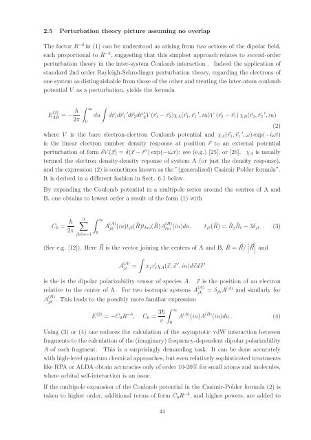
2.5 Perturbation theory picture assuming no overlap
The factor R −6 in (1) can be understood as arising from two actions of the dipolar field,
each proportional to R −3 , suggesting that this simplest approach relates to second-order
perturbation theory in the inter-system Coulomb interaction . Indeed the application of
standard 2nd order Rayleigh-Schrodinger perturbation theory, regarding the electrons of
one system as distinguishable from those of the other and treating the inter-atom coulomb
potential V as a perturbation, yields the formula
E (2)
AB = −
2π
∫ ∞
0
∫
du
d⃗r 1 d⃗r 1 ′ d⃗r 2 d⃗r ′ 2V (⃗r 1 − ⃗r 2 )χ A (⃗r 1 ,⃗r 1 ′ , iu)V (⃗r 2 − ⃗r 1 ) χ B (⃗r 2 ,⃗r 2 ′ , iu)
(2)
where V is the bare electron-electron Coulomb potential and χ A (⃗r 1 ,⃗r 1 ′ , ω) exp(−iωt)
is the linear electron number density response at position ⃗r to an external potential
perturbation of form δV (⃗x) = δ(⃗x − ⃗r ′ ) exp(−iωt): see (e.g.) [25], or [26]. χ A is usually
termed the electron density-density reponse of system A (or just the density response),
and the expression (2) is sometimes known as the ”(generalized) Casimir Polder formula”.
It is derived in a different fashion in Sect. 6.1 below.
By expanding the Coulomb potential in a multipole series around the centres of A and
B, one obtains to lowest order a result of the form (1) with
C 6 =
2π
3∑
jklm=1
∫ ∞
0
A (A)
jk (iu)t jl( ˆR)t (B)
km ( ˆR)A
lm (iu)du, t jl( ˆR) = ˆR j ˆRl − 3δ jl . (3)
(See e.g. [12]). Here R ⃗ is the vector joining the centers of A and B, ˆR = R/ ⃗ ∣R
⃗ ∣ and
∫
A (A)
jl
=
x j x ′ lχ A (⃗x,⃗x ′ , iu)d⃗xd⃗x ′
is the is the dipolar polarizability tensor of species A. ⃗x is the position of an electron
relative to the center of A. For two isotropic systems A (A)
jk
= δ jk A (A) and similarly for
. This leads to the possibly more familiar expression
A (B)
jk
E (2) = −C 6 R −6 ,
C 6 = 3 π
∫ ∞
0
A (A) (iu)A (B) (iu)du . (4)
Using (3) or (4) one reduces the calculation of the asymptotic vdW interaction between
fragments to the calculation of the (imaginary) frequency-dependent dipolar polarizability
A of each fragment. This is a surprisingly demanding task. It can be done accurately
with high-level quantum chemical approaches, but even relatively sophisticated treatments
like RPA or ALDA obtain accuracies only of order 10-20% for small atoms and molecules,
where orbital self-interaction is an issue.
If the multipole expansion of the Coulomb potential in the Casimir-Polder formula (2) is
taken to higher order, additional terms of form C 8 R −8 , and higher powers, are added to
44