Geodesics of the Kerr metric

Chapter 4
Geodesics of the Kerr
metric
Here we will study the geodesic motion outside a Kerr black hole;
therefore, we will only consider the region outside the outer horizon,
r ≥ r + (4.1)
which is the relevant region for astrophysical considerations.
Let us consider a geodesic with affine parameter λ and tangent
vector
u µ = dxµ
dλ ≡ ẋµ (4.2)
in Boyer-Linquist coordinates (we remind that, in our conventions,
the overdot has the meaning of derivation with respect to the affine
parameter λ). The tangent vector u µ is solution of the geodesic
equation
u µ u ν ;µ =0. (4.3)
The geodesic equation (4.3) is equivalent to the Euler-Lagrange
equations
d ∂L
dλ ∂ẋ = ∂L
(4.4)
α ∂x α
associated to the Lagrangian
L (x µ , ẋ µ )= 1 2 g µνẋ µ ẋ ν . (4.5)
One can define the conjugate momentum p µ to the coordinate x µ as
p µ ≡ ∂L
∂ẋ µ = g µνẋ µ . (4.6)
67

In terms of the conjugate momenta, the Euler-Lagrange equations
can be written as
d
dλ p µ = ∂L
∂x . (4.7)
µ
Notice that, if the metric does not depend on a given coordinate x µ ,
the corresponding conjugate momentum is a constant of motion.
The existence of such a constant can also be seen in a simpler way.
We know that, if the metric is independent by a coordinate, there
is a Killing vector ξ µ corresponding to this symmetry, and ξ µ ẋ µ
is a constant of geodesic motion; actually, this constant of motion
coincides with the one arising from Euler-Lagrange equations (as we
will see, for instance, in the case of t and φ for the Kerr metric).
Let us come back to the geodesic equation for Kerr spacetime.
Equation (4.3) (or, equivalently, (4.4)) in Kerr spacetime is very
complicate to solve directly. To study geodesic motion in a simple
way, we would need to find a way to express the geodesic u µ in terms
of conserved quantities, as we have done in the case of Schwarzschild
spacetime. For this, we need four algebraic relations involving u µ .
As we have seen in Section 3.2, Kerr spacetime has two Killing
vectors: a timelike Killing vector k µ =(1, 0, 0, 0) and a spacelike
killing vector m µ =(0, 0, 0, 1). This corresponds to the fact that the
metric (in Boyer-Lindquist coordinates) does not depend explicitly
by t and φ: the spacetime is stationary and axially symmetric.
Therefore, in geodesic motion there are two conserved quantities:
E ≡ −k µ u µ = −g tµ u µ = −p t constant along geodesics
(4.8)
L ≡ m µ u µ = g φµ u µ = p φ constant along geodesics .
(4.9)
As explained in Section 3.2, in the case of massive particle E is the
energy at infinity per mass unit while L is the angular momentum
per mass unit; in the case of massless particles, E is the energy at
infinity and L is the angular momentum.
Furthermore, we have the relation
where
κ = −1
g µν u µ u ν = κ (4.10)
for timelike geodesics
68

κ =1 forspacelikegeodesics
κ =0 fornullgeodesics. (4.11)
The relations (4.8), (4.9), (4.10) give us three algebraic relations
involving u µ ,buttheyarenotsufficienttotodeterminethefour
unknowns u µ . This is different from the case of Schwarzschild spacetime,
where we have the further condition of planarity of the orbit
(u θ (λ) ≡ 0 if θ(λ =0)=π/2 andu θ (λ =0)=0)arisingfromthe
Euler-Lagrange equations, which have a simple form in that case.
Without this further condition, we cannot study geodesic motion
using only (4.8), (4.9), (4.10). Actually, there is a further conserved
quantity, the Carter constant, whichallowstofindthetangentvector
u µ through algebraic relations.
Anyway, it is possible to study geodesic motion with the only help
of (4.8), (4.9), (4.10) in the particular case of equatorial motion, i.e.
with θ ≡ π/2. Therefore, we will first study equatorial geodesics,
and then, in Section 4.2, we will consider the case of general motion
and derive the Carter constant.
4.1 Equatorial geodesics
In this section we study equatorial geodesics, i.e. geodesics with
θ ≡ π 2 . (4.12)
First of all, let us prove that such geodesics exist, i.e. that equatorial
geodesics are solutions of the geodesic equation (4.3), or, equivalently,
of the Euler-Lagrange equations (4.4). The θ component of
(4.4) is
d
dλ (g θµẋ µ )= d
dλ (Σ ˙θ) =Σ¨θ +Σ ,µ ẋ µ 1
˙θ =
2 g µν,θẋ µ ẋ ν (4.13)
where we have used the fact that the only non-vanishing g θµ component
in (3.1) is g θθ =Σ.
The right-hand side is
( )
(ṙ)
g µν,θ ẋ µ ẋ ν 2
=Σ ,θ
∆ +(˙θ) 2 + 2 sin θ cos θ(r 2 + a 2 )( ˙φ) 2
−
2Mr (
Σ Σ 2 ,θ a sin 2 θ ˙φ
) 2 4Mr
(
− ṫ + a sin 2 θ
Σ
˙φ
)
− ṫ 2a sin θ cos θ ˙φ
(4.14)
69

where Σ ,θ = −2a 2 sin θ cos θ and Σ ,r =2r. It is easy to check that
θ ≡ π/2 is a solution of equation (4.13).
If, at λ = 0, the particles moves in the equatorial plane, θ(λ =
0) = π/2 and ˙θ(λ =0)=0;thenwehaveawell-posedCauchy
problem of the form
¨θ = ...
˙θ(λ =0) = 0
θ(λ =0) = π 2
(4.15)
which admits one and only one solution; since θ ≡ π/2 is a solution,
it is the solution. Thus, a geodesic which starts in the equatorial
plane, remains in the equatorial plane.
This also happens in the Schwarzschild metric. But, while in that
case it is possible to generalize the result to any orbit, thanks to the
spherical symmetry, and prove that allSchwarzschildgeodesicsare
planar, such a generalization is not possible for the Kerr metric
which is axially symmetric. We only can say that geodesics starting
in the equatorial plane are planar.
On the equatorial plane, Σ = r 2 ,therefore
(
g tt = − 1 − 2M )
r
and
E = −g tµ u µ =
g tφ = − 2Ma
r
g rr = r2
∆
g φφ = r 2 + a 2 + 2Ma2
r
(
1 − 2M r
L = g φµ u µ = − 2Ma ṫ +
r
(4.16)
)
ṫ + 2Ma ˙φ (4.17)
r
)
(r 2 + a 2 + 2Ma2 ˙φ. (4.18)
r
To solve (4.17), (4.18) for ṫ, ˙φ we define
A ≡ 1 − 2M r
70

B ≡ 2Ma
r
C ≡ r 2 + a 2 + 2Ma2
r
so that (4.17), (4.18) can be written as
We also have
Therefore,
i.e.
AC + B 2 =
(4.19)
E = Aṫ + B ˙φ (4.20)
L = −Bṫ + C ˙φ. (4.21)
(
1 − 2M r
) )(r 2 + a 2 + 2Ma2 + 4M 2 a 2
r r 2
= r 2 − 2Mr + a 2 =∆. (4.22)
CE − BL = [AC + B 2 ]ṫ =∆ṫ
AL + BE = [AC + B 2 ] ˙φ =∆˙φ (4.23)
ṫ = 1 )
[(r 2 + a 2 + 2Ma2 E − 2Ma ]
L
∆
r r
˙φ = 1 [(
1 − 2M )
L + 2Ma ]
E . (4.24)
∆ r r
Equation (4.10) can be written in terms of A, B, C:
g µν u µ u ν = κ
= −Aṫ 2 − 2Bṫ ˙φ + C ˙φ 2 + r2
∆ ṙ2
= −[Aṫ + B ˙φ]ṫ +[−Bṫ + C ˙φ] ˙φ + r2
∆ ṙ2
= −Eṫ + L ˙φ + r2
∆ ṙ2 (4.25)
where we have used (4.20), (4.21). Therefore,
ṙ 2 = ∆ r 2 (Eṫ − L ˙φ + κ)
= 1 r 2 [
CE 2 − 2BLE − AL 2] + κ∆
r 2
= C r 2 (E − V +)(E − V − )+ κ∆
r 2 (4.26)
71

where V ± (r) are the solutions of the equation in E
i.e.
V ± = BL ± √ B 2 L 2 + ACL 2
C
CE 2 − 2BLE − AL 2 =0, (4.27)
= 1 C (BL ±|L|√ ∆) . (4.28)
Some authors write this formula without the modulus (which is
equivalent to exchange the definitions of V + and V − when L 0, C>0.
In the Schwarzschild limit a → 0, we have
V + + V − ∝ a → 0 ,
V + V − →− L2 ∆
r 4 (4.32)
therefore, if we define V ≡−V + V − − κ∆/r 2 ,Eqns. (4.30),(4.31)
reduce to the well known form
ṙ 2 = E 2 − V (r)
V (r) = − κ∆
r + L2 ∆
(
2 r 4
= 1 − 2M )
)(−κ + L2
r
r 2
(4.33)
where we recall that κ = −1 fortimelikegeodesics,κ = 0 for null
geodesics, κ =1forspacelikegeodesics.
72

4.1.1 Null geodesics
In the case of null geodesics (4.30) becomes
with
ṙ 2 = (r2 + a 2 ) 2 − a 2 ∆
r 4 (E − V + )(E − V − ) (4.34)
V ± = 2MLar ±|L|r2√ ∆
(r 2 + a 2 ) 2 − a 2 ∆ . (4.35)
We have two possibilities: La > 0andLa < 0, i.e. the photon and
the black hole corotating and counterrotating; notice that we always
have
V + ≥ V − . (4.36)
Since ṙ 2 must be positive, from eq. (4.34) we see that, being (r 2 +
a 2 ) 2 − a 2 ∆ > 0, null geodesics are possible for massless particle
whose constant of motion E satisfies the following inequalities
EV + . (4.37)
Thus, the region V − 0andthenV + >V − .Furthermore,
V + (r + )=V − (r + )= 2Mr +La
(r 2 + + a 2 ) 2 = LΩ H , (4.39)
which is positive if La > 0, negative if La < 0.
• In the limit r →∞, V ± → 0.
• If La > 0(corotatingorbits),thepotentialV + is definite positive;
V − (which is positive at r + )vanisheswhen
r √ ∆=2M|a| ⇒ r 2 (r 2 − 2Mr + a 2 )=4M 2 a 2 (4.40)
which gives
r 4 − 2Mr 3 + a 2 r 2 − 4M 2 a 2 =(r − 2M)(r 3 + a 2 r +2Ma 2 )=0;
(4.41)
thus V − vanishes at r =2M, which is the location of the ergosphere
in the equatorial plane (r S+ (θ = π/2) = 2M).
73

• If La < 0(counterrotatingorbits),thepotentialV − is definite
negative and V + (which is negative at r + )vanishesatthe
ergosphere r = r S+ =2M.
• The study of the derivatives of V ± , which is too long to be
reported here, tells us that both potentials, V + and V − ,have
only one stationary point.
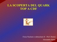
In summary, V + (r) andV − (r) have the shapes shown in Figure 4.1
where in the two panels we show the cases La > 0(up)andLa < 0
(down), respectively. Once we have drawn the curves V + (r),V − (r)
L
V
V
r + r S+
La > 0
V +
V
La < 0
V +
r r + S+
r
r
L
V
Figure 4.1: The potentials V + (r) andV − (r), for corotating (La > 0) and counterrotating
(La < 0) orbits. The shadowed region is not accessible to the motion
of photons or other massless particles.
for assigned values of a, M and L, wecanmakeaqualitativestudy
74

of the orbits. To this purpose it is useful to compute the radial
acceleration. By differentiating eq. (4.34)
(ṙ) 2 = C r (E − V +)(E − V 2 − ) (4.42)
with respect to the geodesic parameter λ, wefind
2ṙ¨r =
[( ) ′ C
(E − V
r 2 + )(E − V − ) − C r V +(E ′ − V 2 − )
− C ]
r V ′ 2 − (E − V +) ṙ (4.43)
i.e.
¨r = 1 ( ) ′ C
(E − V
2 r 2 + )(E − V − ) − C [
V
′
2r 2 + (E − V −)+V − ′ (E − V +) ] .
(4.44)
Let us consider the radial acceleration in a point where the radial
velocity ṙ is zero, i.e. when E = V + or E = V − :
Since
we find
¨r = − C
2r V ′ 2 + (V + − V − ) if E = V +
¨r = − C
2r V ′ 2 − (V − − V + ) if E = V − . (4.45)
V + − V − =
2|L|r 2√ ∆
(r 2 + a 2 ) 2 − a 2 ∆ = 2|L|√ ∆
, (4.46)
C
¨r = ∓ |L|√ ∆
r 2 V ′ ± if E = V ± . (4.47)
This result shows that if, for example, E = V + (r max )wherer max is
astationarypointforV + (i.e. V ′ + (r max) =0),theradialacceleration
vanishes; since when E = V + (r max )theradialvelocityalsovanishes,
a massless particle with that value of E can be captured on a circular
orbit, but the orbit is unstable, as it is the orbit at r =3M for the
Schwarzschild metric.
It is possible to show that r max is the solution of the equation
r(r − 3M) 2 − 4Ma 2 =0. (4.48)
75

Note that this equation does not depend on L, thusthevalueofr max
is independent of L. The solution of (4.48) is a decreasing function
of a, and,inparticular,
r max = 3M for a =0
r max = M for a = M
r max = 4M for a = −M . (4.49)
Therefore, while for a Schwarzschild black hole the unstable circular
orbit for a photon is located at r = 3M, for a Kerr black hole
it can be located much closer to the black hole, in particular for
large values of a; in the case of an extremal (a = M) blackhole,
r max = M, whichisthepositionofthehorizonforsuchablackhole
(see also Figure 4.2).
A photon coming from infinity with constant of motion E >
V + (r max ), falls inside the horizon, whereas if 0 0.
It remains to consider the case when E

ackwards in time. Furthermore, from a quantum-mechanical point
of view, the existence of negative energy particle states would lead
to an unstable vacuum, since it would be energetically favourable
the creation of more and more of such particles.
The energy measured by a different observer is different, but its
sign is the same: indeed, if u µ =(γ,γV) withγ =(1− V 2 ) −1/2 ,
then
E (u) = −γ(P 0 + P i V i ) (4.51)
which has the same sign as −P 0 since |P i V i | < |P 0 |.Wecanconclude
that, in special relativity, particles must have positive energy with
respect to all observers; and that if the energy is positive as measured
by any observer (for instance the static observer), it is positive as
measured by all observers.
In general relativity, we still define the energy of a particle measured
by an observer u µ as in eq. (4.50). Indeed, eq. (4.50) is a
tensor equation which holds in a locally inertial frame, and consequently
in any other frame by the principle of general covariance.
For the same reason, it must be
E (u) > 0 , (4.52)
and it is sufficient to prove this for any observer.
Let us now consider a particle in the Kerr spacetime, located
at radial infinity (where a static observer with u µ st =(1, 0, 0, 0) can
always be defined). According to the definition E (u) = −u µ P µ ,the
energy measured by the static observer will be E (ust) = −P 0 and,
according to eq. (3.21) 1 E (ust) = −P 0 = E (4.53)
We conclude that for a particle coming from radial infinity, the
constant of motion E can be identified with the energy as measured
by a static observer at infinity, and consequently orbits with negative
values of E are not allowed.
Referring to figure 4.1, let us now consider a massless particle,
say a photon, that moves in the ergoregion, i.e. between r + and r S+ .
A static observer cannot exist in this region, therefore we need to
consider a different observer, for instance the ZAMO,
u µ ZAMO
= C(1, 0, 0, Ω) (4.54)
1 Note that eq. (4.53) holds for a massless particle; in the case of a massive particle, where
E is the energy at infinity per mass unit, we have to multiply E with the particle mass.
77

where (see eq. (3.29) )
Ω=
2Mar
(r 2 + a 2 ) 2 − a 2 ∆
(4.55)
and C is found by imposing g µν u µ ZAMO uν ZAMO = −1. We have C>0,
otherwise the ZAMO would move backwards in time.
The energy of the photon with respect to the ZAMO is
E ZAMO = −P µ u µ ZAMO
= C(E − ΩL) . (4.56)
Thus, the requirement E ZAMO > 0 is equivalent to
E>ΩL. (4.57)
Notice that, by comparing (4.55) with (4.35) we find that
V − < ΩL V + satisfy (4.57), have positive
energies with respect to the ZAMO, and are then allowed. The
geodesics with EV + (4.59)
(necessary and sufficient to have a particle with positive energy E)
allows negative values of the constant of motion E. This is not a
contradiction, because it is only at infinity that E represents the
physical energy of the particle; the geodesics we are considering
never reach infinity.
We can conclude that the constant E (which is the energy at
infinity) must always be larger than V +
E>V + (r) (4.60)
and this guarantees that the energy of the particle, as measured by
a local observer, is positive; in the counterrotating case La < 0, E
can be negative still preserving (4.60), because inside the ergosphere
V + < 0.
78

4.1.3 The Penrose process
A short comment about notation: in this section we will use a
slightly different notation for the constants of motion E, L, which
have been defined in Section 3.2 to be the energy at infinity and
angular momentum per unit mass in the case of massive particles,
and to be the energy at infinity and angular momentum in the case
of massless particles, namely,
E = −k µ u µ , L = m µ u µ . (4.61)
Here (only in this Section) we define E,L to be the energy at infinity
and the angular momentum, both for massive and massless particles,
i.e.
E = −k µ P µ , L = m µ P µ . (4.62)
This means that we have multiplied E and L, in the case of massive
particles, with the mass m.
After this premise, let us consider an interesting consequence
of the possibility of having particles moving with negative E: it is
possible to extract rotational energy from a Kerr black hole, through
amechanismcalledPenrose process.
Let us assume that the black hole has a>0. The same reasoning
can be repeated in the case of a

contracting with −k µ and with m µ we find
E = E 1 + E 2
L = L 1 + L 2 . (4.67)
We also assume that the particle 1 is massless (i.e. a photon), and
that ṙ 1 < 0andṙ 2 > 0: the particle 1 falls in the black hole, while
the particle 2 comes back to infinity.
The photon 1 never goes outside the ergosphere, thus we can
require E 1 < 0, if L 1 < 0. Then, it must be
and the particle 2 reaches infinity with
V − (r + )(= V + (r + )) E
L 2 = L − L 1 >L. (4.69)
In this way, at the end we have at infinity a particle more energetic
than the initial one. We say we have extracted rotational energy from
the black hole because the photon 1, with E 1 < 0,L 1 < 0, reduces
the mass-energy M of the black hole and its angular momentum
J = Ma to the values M fin , J fin respectively:
M fin = M + E 1

If we compute the integral at a time when the particle is far away
from the black hole, then the spacetime is flat where Tparticle
00 ≠
0; the stress-energy tensor for a point particle with energy E, in
Minkowskian coordinates, has
Integrating in V we get
T 00
particle = Eδ3 (x − x(t)) . (4.74)
P 0
tot = E + M (4.75)
computed when the initial particle is still far away from the black
hole.
On the other hand, this quantity is conserved, because [(−g)(T 0µ +
t 0µ )] ,µ =0impliesPtot 0
,0 =0,sinceweneglecttheoutgoinggravitational
flux generated by the particle. Therefore, repeating the computation
when the particle 2 has reached infinity, when the mass of
the black hole is M fin ,
P 0
tot = E 2 + M fin . (4.76)
This proves the relation (4.70). A similar proof holds for the angular
momentum.
4.1.4 The innermost stable circular orbit for timelike geodesics
The study of timelike geodesics is much more complicate, because
equation (4.26), which becomes when κ = −1
ṙ 2 = C r 2 (E − V +)(E − V − ) − ∆ r 2 , (4.77)
does not allow a simple qualitative study as in the case of null
geodesics. Therefore, here we only report on some results one finds
by a detailed study of these equations.
A very relevant quantity (with astrophysical interest) is the location
of the innermost stable circular orbit (ISCO), which, in the
Schwarzschild case, is at r =6M. InKerrspacetime,theexpression
for r ISCO is quite complicate, but its qualitative behaviour is simple:
there are two solutions
r ± ISCO
(a) , (4.78)
one corresponding to corotating orbits, one to counterrotating orbits.
For a =0,obviouslythetwosolutionscoincideto6M; by
81

increasing |a|, theISCOmovesclosertotheblackholeforcorotating
orbits, and far away from the black hole for counterrotating
orbits. When a = ±M, the ISCO, in the corotating case, coincides
with the horizon, at r = M. Thisbehaviourisverysimilartothat
we have already seen in the case of unstable circular orbits for null
geodesics.
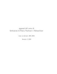
In Figure 4.2 we show (in the case a ≥ 0) the locations of the
last stable and unstable circular orbits for timelike geodesics, and
of the unstable circular orbit for null geodesics. This figure is taken
from the article where these orbits have been studied (J. Bardeen,
W. H. Press, S. A. Teukolsky, Astrophys. J. 178, 347, 1972).
4.1.5 The 3 rd Kepler law
Let us consider a circular timelike geodesic in the equatorial plane.
We remind that the Lagrangian (4.5) is
and the r Euler-Lagrange equation is
L = 1 2 g µνẋ µ ẋ ν (4.79)
d ∂L
dλ ∂ṙ = ∂L
∂r . (4.80)
Being g rµ = 0 if µ ≠ r, wehave
d
dλ (g rrṙ) = 1 2 g µν,rẋ µ ẋ ν . (4.81)
In the case of a circular geodesic, ṙ = ¨r = 0, and this equation
reduces to
g tt,r ṫ 2 +2g tφ,r ṫ ˙φ + g φφ,r ˙φ2 =0. (4.82)
The angular velocity is ω = ˙φ/ṫ, thus
We remind that
g φφ,r ω 2 +2g tφ,r ω + g tt,r =0. (4.83)
g tt = −
(
1 − 2M r
g tφ = − 2Ma
r
)
g φφ = r 2 + a 2 + 2Ma2
r
82
, (4.84)

Figure 4.2: Geodesics of Massive particles in Kerr metric, from Bardeen et al.,
Astrophys. J. 178, 347, 1972.
83

then
The equation
)
2
(r − Ma2 ω 2 + 4Ma ω − 2M =0. (4.85)
r 2 r 2 r 2
(r 3 − Ma 2 )ω 2 +2Maω − M =0 (4.86)
has discriminant
M 2 a 2 + M(r 3 − Ma 2 )=Mr 3 (4.87)
and solutions
ω ± = −Ma ± √ Mr 3
= ± √ M r3/2 ∓ a √ M
r 3 − Ma 2
r 3 − Ma 2
= ± √ r 3/2 ∓ a √ M
M
(r 3/2 + a √ M)(r 3/2 − a √ M)
√
M
= ±
r 3/2 ± a √ M . (4.88)
This is the relation between angular velocity and radius of circular
orbits, and reduces, in Schwarzschild limit a =0,to
which is Kepler’s 3 rd law.
ω ± = ±√
M
r 3 , (4.89)
4.2 General geodesic motion: the Carter constant
To study generic geodesics in Kerr spacetime, we need to apply
the Hamilton-Jacobi approach, whichallowstoidentifyafurther
constant of motion (not related to anyisometryofthemetric).
To apply the Hamilton-Jacobi approach, we first have to express
our system with an Hamiltonian description. Given the Lagrangian
of the system
L(x µ , ẋ µ )= 1 2 g µνẋ µ ẋ ν (4.90)
84

we have defined the conjugate momenta 2
p µ = ∂L
∂ẋ µ = g µνẋ ν . (4.91)
By inverting (4.91), we can express ẋ µ in terms of the conjugate
momenta:
ẋ µ = g µν p ν . (4.92)
The Hamiltonian is a functional of the coordinate functions x µ (λ)
and of their conjugate momenta p µ (λ), defined as
In our case, we have
H(x µ ,p ν )=p µ ẋ µ (p ν ) −L(x µ , ẋ µ (p ν )) . (4.93)
H = 1 2 gµν p µ p ν . (4.94)
The geodesics equation is equivalent to the Euler-Lagrange equations
for the Lagrangian functional, which are equivalent to the
Hamilton equations for the Hamiltonian functional:
ẋ µ = ∂H
∂p µ
ṗ µ = − ∂H
∂x µ . (4.95)
To solve equations (4.95) is as difficult as to solve the Euler-Lagrange
equations. Anyway, it is possible to apply the Hamilton-Jacobi approach,
which here we briefly recall.
In the Hamilton-Jacobi approach, we look for a function of the
coordinates and of the curve parameter λ,
S = S(x µ ,λ) (4.96)
which is solution of the Hamilton-Jacobi equation
(
H x µ , ∂S )
+ ∂S =0. (4.97)
∂x µ ∂λ
In general such a solution will depend on four integration constants.
It can be shown that, if S is a solution of the Hamilton-Jacobi
equation, then
∂S
∂x µ = p µ . (4.98)
2 Not to be confused with the four-momentum of the particle, which we denote with P µ .
85

Therefore, once we have solved (4.97), we have the expressions of
the conjugate momenta (and then of ẋ µ ) in terms of four constants,
which allow to write the solutions of the geodesic equation in a
closed form, in terms of integrals.
In general, it is more difficult to solve (4.97), which is a partial
differential equation, than to solve thegeodesicequation,butinthis
case we can find such a solution.
First of all, we can use what we already know, i.e.
These conditions require that
H = 1 2 gµν p µ p ν = 1 2 κ
p t = −E constant
p φ = L constant . (4.99)
S = − 1 2 κλ − Et + Lφ + S(rθ) (r, θ) (4.100)
where S (rθ) is a function of r and θ to be determined.
Furthermore, we look for a separable solution, by making the
ansatz
S = − 1 2 κλ − Et + Lφ + S(r) (r)+S (θ) (θ) . (4.101)
Substituting (4.101) into the Hamilton-Jacobi equation (4.97), and
using the expression (3.16) for the inverse metric, we find
−κ + ∆ ( ) dS
(r) 2
+ 1 ( ) dS
(θ) 2
Σ dr Σ dθ
− 1 ]
[r 2 + a 2 + 2Mra2
∆
Σ
sin2 θ E 2 + 4Mra
Σ∆ EL + ∆ − a2 sin 2 θ
Σ∆ sin 2 θ L2 =0.
(4.102)
Using the relation (3.12)
(r 2 + a 2 )+ 2Mra2
Σ
sin2 θ = 1 Σ
and multiplying by Σ = r 2 + a 2 cos 2 θ,weget
( ) dS
−κ(r 2 + a 2 cos 2 (r) 2 ( dS
(θ)
θ)+∆ +
dr dθ
[
(r 2 + a 2 ) 2 − a 2 sin 2 θ∆ ] (4.103)
86
) 2

[ ]
(r 2 + a 2 ) 2
−
− a 2 sin 2 θ E 2 + 4Mra ( ) 1
∆
∆ EL + sin 2 θ − a2
L 2 =0
∆
(4.104)
i.e.
( ) dS
(r) 2
∆ − κr 2 − (r2 + a 2 ) 2
E 2 + 4Mra a2
EL −
dr
∆
∆ ∆ L2
( ) dS
(θ) 2
= − + κa 2 cos 2 θ − a 2 sin 2 θE 2 − 1
dθ
sin 2 θ L2 .
(4.105)
We rearrange equation (4.105) by adding to both sides the constant
quantity a 2 E 2 + L 2 :
( ) dS
(r) 2
∆ − κr 2 − (r2 + a 2 ) 2
E 2 + 4Mra a2
EL −
dr
( dS
(θ)
= −
dθ
∆
∆
) 2
+ κa 2 cos 2 θ + a 2 cos 2 θE 2 − cos2 θ
sin 2 θ L2 .
∆ L2 + a 2 E 2 + L 2
(4.106)
In equation (4.106), the left-hand side does not depend on θ, and it
is equal to the right-hand side which does not depend on r; therefore,
this quantity must be a constant C:
( ) dS
(θ) 2 [
− cos 2 θ (κ + E 2 )a 2 − 1 ]
dθ
sin 2 θ L2 = C
( ) dS
(r) 2
∆ − κr 2 − (r2 + a 2 ) 2
E 2 + 4Mra a2
EL −
dr
∆
∆ ∆ L2 + E 2 a 2 + L 2
( ) dS
(r) 2
= ∆ − κr 2 +(L − aE) 2 − 1 [
E(r 2 + a 2 ) − La ] 2
= −C .
dr
∆
(4.107)
Notice that in rearranging the terms between the last two lines, we
have used, for the LE terms, the relation
−2aLE +2aLE r2 + a 2
∆
= 4aMr LE . (4.108)
∆
87

If we define the functions R(r) andΘ(θ) as
[
Θ(θ) ≡ C +cos 2 θ (κ + E 2 )a 2 − 1 ]
sin 2 θ L2
then
R(r) ≡ ∆ [ −C + κr 2 − (L − aE) 2] + [ E(r 2 + a 2 ) − La ] 2
,
(4.109)
( ) dS
(θ) 2
= Θ
dθ
( ) dS
(r) 2
= R (4.110)
∆ 2
dr
and the solution of the Hamilton-Jacobi equation has the form
S = − 1 2 κλ − Et + Lφ + ∫ √
R
∆ dr + ∫ √Θdθ
. (4.111)
Once we have the solution of the Hamilton-Jacobi equations, depending
on four constants (κ, E, L, C), it is possible to solve the
geodesic motion. Indeed, from (4.98) we know the expressions of
the conjugate momenta
therefore
p 2 θ = (Σ˙θ) 2 =Θ(θ)
( ) 2 Σ
p 2 r = = R(r)
(4.112)
∆ṙ ∆ 2
˙θ = ± 1 Σ√
Θ
ṙ = ± 1 Σ√
R (4.113)
which can be solved by simple integration. The constant C is called
Carter constant, and characterize, together with E and L, the geodesic
motion. Notice that differently from E and L, theCarterconstant
is not related to any isometry of the spacetime.
To integrate equations (4.113), it is convenient to define a new
variable λ ′ to parametrize the geodesic, called “Mino time”:
dλ =Σdλ ′ =(r 2 + a 2 cos 2 θ)dλ ′ . (4.114)
88

Then we have
dθ
dλ ′ = ± √ Θ(θ)
dr
dλ ′ = ± √ R(r) , (4.115)
thus the equations for r and θ, once expressed in the Mino time, are
decoupled. An important consequence of this property is that for
bound orbits, which satisfy R(r) > 0forr 1