Decentralization and Corruption in the Philippines
Decentralization and Corruption in the Philippines
Decentralization and Corruption in the Philippines

Create successful ePaper yourself
Turn your PDF publications into a flip-book with our unique Google optimized e-Paper software.
L:\IrisPhilipp<strong>in</strong>es\Paper\<strong>Decentralization</strong> <strong>and</strong> corruption <strong>in</strong> <strong>the</strong> Philipp<strong>in</strong>es July 16.doc<br />
Very Prelim<strong>in</strong>ary, not for circulation<br />
<strong>Decentralization</strong> <strong>and</strong> <strong>Corruption</strong> <strong>in</strong> <strong>the</strong> Philipp<strong>in</strong>es<br />
Omar Azfar <strong>and</strong> Tugrul Gurgur *<br />
* omar@iris.econ.umd.edu; tgurgur@worldbank.org
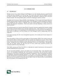
I. Introduction<br />
When Corazon Aqu<strong>in</strong>o toppled <strong>the</strong> <strong>in</strong>famously corrupt regime of Ferd<strong>in</strong><strong>and</strong> Marcos<br />
<strong>in</strong> <strong>the</strong> democratic revolution of 1986, she promised to follow <strong>the</strong> democratization with a<br />
far-reach<strong>in</strong>g devolution of political <strong>and</strong> adm<strong>in</strong>istrative authority to <strong>the</strong> local level. The<br />
revolutionary government made good on its promise <strong>and</strong> <strong>the</strong> Local Governments Act of<br />
1991 devolved both political authority <strong>and</strong> adm<strong>in</strong>istrative control of many health services<br />
<strong>and</strong> o<strong>the</strong>r subjects to <strong>the</strong> prov<strong>in</strong>cial <strong>and</strong> municipal level. In this paper we exam<strong>in</strong>e <strong>the</strong><br />
causes <strong>and</strong> consequences of corruption at <strong>the</strong> local level <strong>in</strong> <strong>the</strong> Philipp<strong>in</strong>es with a focus<br />
on health services.<br />
The devolution of authority <strong>in</strong> <strong>the</strong> Philipp<strong>in</strong>es was serious 1 . The Local<br />
Government Code enacted <strong>in</strong> 1991 <strong>and</strong> implemented <strong>in</strong> 1992-3 significantly <strong>in</strong>creased <strong>the</strong><br />
responsibilities <strong>and</strong> resources of sub-national governments: 77 prov<strong>in</strong>ces, 72 cities, 1526<br />
municipalities <strong>and</strong> over 40,000 barangays 2 . To defray <strong>the</strong> cost of devolved expenditures,<br />
Section 284 of <strong>the</strong> Local Government Code provided for 40 percent of central<br />
government revenues collected three years before to be transferred back to sub-national<br />
governments as <strong>in</strong>ternal revenue allotments (IRAs) 3 . Prov<strong>in</strong>ces <strong>and</strong> cities received 23<br />
percent each of <strong>the</strong> total transfer, municipalities 24 percent <strong>and</strong> barangays 20 percent.<br />
Prov<strong>in</strong>ces also received limited new tax<strong>in</strong>g authority over local natural resource<br />
exploitation, agriculture, <strong>and</strong> o<strong>the</strong>r bus<strong>in</strong>ess activities. In addition, <strong>the</strong> Local Government<br />
Code m<strong>and</strong>ated <strong>the</strong> creation of local democracies at each level, with regular elections<br />
be<strong>in</strong>g held for both executives <strong>and</strong> legislative bodies. The comb<strong>in</strong>ation of <strong>the</strong> devolution<br />
of real expenditure authority, substantial transfers to local governments so <strong>the</strong>y can<br />
implement many of <strong>the</strong>ir m<strong>and</strong>ates, <strong>and</strong> <strong>the</strong> creation of a vibrant local democracy makes<br />
it fair to call <strong>the</strong> decentralization <strong>in</strong> <strong>the</strong> Philipp<strong>in</strong>es <strong>in</strong> <strong>the</strong> early 1990’s a serious<br />
devolution.<br />
The Philipp<strong>in</strong>es cont<strong>in</strong>ues to be a highly corrupt country ranked 69 out of 90<br />
nations by Transparency International. The President has recently been impeached on a<br />
corruption count <strong>and</strong> removed from office <strong>in</strong> a case that <strong>in</strong>volves local level corruption<br />
1 The next few paragraphs borrow heavily from Ma<strong>the</strong>son <strong>and</strong> Azfar 1999. See Meagher 2000 for a detailed<br />
<strong>in</strong>stitutional analysis of decentralization <strong>in</strong> <strong>the</strong> Philipp<strong>in</strong>es.<br />
2 These numbers change as new units are created or old ones comb<strong>in</strong>ed (Miller 1997)<br />
2
with kickbacks passed up to <strong>the</strong> Presidency. Much of <strong>the</strong> corruption <strong>in</strong> <strong>the</strong> Philipp<strong>in</strong>es<br />
does appear to be at <strong>the</strong> local level, of <strong>the</strong> 336 impend<strong>in</strong>g corruption cases, 49% are<br />
aga<strong>in</strong>st municipal mayors- <strong>the</strong> level of government which is our focus <strong>in</strong> this study<br />
(Batalla 2000). Many observers have stated that corruption is <strong>the</strong> root cause of cont<strong>in</strong>ued<br />
poverty <strong>in</strong> <strong>the</strong> Philipp<strong>in</strong>es. All this makes our study of local level corruption <strong>in</strong> <strong>the</strong><br />
Philipp<strong>in</strong>es highly relevant <strong>in</strong> a country specific context.<br />
In addition studies such as this one might have global relevance <strong>in</strong> terms of <strong>the</strong><br />
<strong>in</strong>creas<strong>in</strong>gly important question of <strong>the</strong> determ<strong>in</strong>ants of local government performance <strong>and</strong><br />
<strong>the</strong> effect of corruption on health service delivery. However, we acknowledge <strong>the</strong><br />
difficulty of generaliz<strong>in</strong>g from one possibly unrepresentative country, <strong>and</strong> would prefer to<br />
replicate this study <strong>in</strong> o<strong>the</strong>r countries with a large number of local governments before<br />
mak<strong>in</strong>g global prescriptions.<br />
It is important to po<strong>in</strong>t out one related question that our study does not answer: <strong>the</strong><br />
impact of decentralization on corruption. The decentralization <strong>in</strong> <strong>the</strong> Philipp<strong>in</strong>es did<br />
co<strong>in</strong>cide with an improvement <strong>in</strong> corruption assessments by <strong>the</strong> International Country<br />
Risk Guide produced by Political Services International (Figure 1), but this could be due<br />
to any number of reasons (<strong>the</strong>re was also a change of government around this time), <strong>and</strong><br />
its difficult to say anyth<strong>in</strong>g more. There is reportedly more corruption at <strong>the</strong> national<br />
level accord<strong>in</strong>g to our respondents –<strong>the</strong> most reliable respondents for this comparison<br />
may be private school pr<strong>in</strong>cipals (Table 1)- but this could easily be due to <strong>the</strong>re be<strong>in</strong>g<br />
more opportunities for corruption at <strong>the</strong> national level which controls more than 80% of<br />
Philipp<strong>in</strong>e f<strong>in</strong>ances. As we can see <strong>in</strong> Figure 2, <strong>the</strong> extent of authority <strong>in</strong> different<br />
branches of government does correspond with levels of corruption, though <strong>the</strong> extremely<br />
small sample size does not allow any authoritative statements. We exam<strong>in</strong>e this issue<br />
below <strong>in</strong> some detail us<strong>in</strong>g variation across municipalities.<br />
This paper is structured as follows. We beg<strong>in</strong> by describ<strong>in</strong>g <strong>the</strong> data. In particular<br />
we exam<strong>in</strong>e <strong>in</strong> detail <strong>the</strong> quality of <strong>the</strong> data on corruption <strong>and</strong> are reassured by a number<br />
of correlations across samples. The corruption perceptions of households, municipal<br />
adm<strong>in</strong>istrators <strong>and</strong> municipal health officers are all correlated with each o<strong>the</strong>r <strong>and</strong> <strong>the</strong><br />
3 The large discrepancy between <strong>the</strong> 40% revenue allotments <strong>and</strong> <strong>the</strong> 12.6% of devolved expenditures can<br />
be expla<strong>in</strong>ed <strong>in</strong> part by <strong>the</strong> three-year lag <strong>and</strong> unbalanced budgets.<br />
3
corruption perceptions of households are highly correlated with <strong>the</strong> corruption<br />
perceptions of o<strong>the</strong>r households <strong>in</strong> <strong>the</strong>ir municipality.<br />
Emboldened by <strong>the</strong>se f<strong>in</strong>d<strong>in</strong>gs, we beg<strong>in</strong> to exam<strong>in</strong>e first <strong>the</strong> causes <strong>and</strong> <strong>the</strong>n <strong>the</strong><br />
consequences of corruption. We f<strong>in</strong>d strong evidence that vot<strong>in</strong>g <strong>in</strong> local elections is<br />
related to lower corruption <strong>and</strong> weaker evidence that read<strong>in</strong>g national newspapers is<br />
related to less corruption. However read<strong>in</strong>g local newspapers has an apparently perverse<br />
effect on corruption.<br />
We also some f<strong>in</strong>d evidence for <strong>the</strong> hypo<strong>the</strong>sis that <strong>in</strong>creases <strong>in</strong> discretion enjoyed<br />
by local governments lead to <strong>in</strong>creases <strong>in</strong> local level corruption (Myrdal 1968, Klitgaard<br />
1988). More extensive decentralization, which would <strong>in</strong>crease discretion at <strong>the</strong> local<br />
level while decreas<strong>in</strong>g it at <strong>the</strong> national level, may merely shift opportunities for<br />
corruption <strong>and</strong> corruption itself from <strong>the</strong> central to <strong>the</strong> local government. Tak<strong>in</strong>g <strong>the</strong><br />
example of <strong>the</strong> sc<strong>and</strong>al that led to <strong>the</strong> removal of president Estrada, had <strong>the</strong> local<br />
government not required <strong>the</strong> assent of someone at <strong>the</strong> center to <strong>in</strong>dulge <strong>in</strong> <strong>the</strong> alleged<br />
improprieties it seems likely that money would still have changed h<strong>and</strong>s <strong>and</strong> <strong>the</strong><br />
gambl<strong>in</strong>g allowed, but <strong>the</strong> money wouldn’t have been shared with <strong>the</strong> center.<br />
We next turn to <strong>the</strong> consequences of corruption. Here we use several different<br />
outcome measures from different sources. We use answers to a test of knowledge<br />
question we adm<strong>in</strong>istered to officials; households reports of wait<strong>in</strong>g time <strong>and</strong> <strong>the</strong>ir<br />
satisfaction with government health services; <strong>and</strong> <strong>in</strong>creases <strong>in</strong> immunizations <strong>and</strong><br />
decreases <strong>in</strong> <strong>in</strong>fectious diseases. In each case we f<strong>in</strong>d <strong>the</strong> expected negative, <strong>and</strong> often<br />
significant, effect of corruption on performance. We also f<strong>in</strong>d a number of <strong>in</strong>terest<strong>in</strong>g<br />
<strong>in</strong>terrelationships between performance variables like <strong>the</strong> importance of knowledge of<br />
immunizations for o<strong>the</strong>r reductions <strong>in</strong> measles <strong>and</strong> o<strong>the</strong>r <strong>in</strong>fectious diseases. Out results<br />
for education are slightly weaker. We do f<strong>in</strong>d a significant negative effect on household<br />
assessments of satisfaction with schools but only an <strong>in</strong>significant effect on test cores. It<br />
is possible however that this last <strong>in</strong>significant result is caused by <strong>the</strong> large number of<br />
miss<strong>in</strong>g observations for test scores.<br />
In summary, we f<strong>in</strong>d that political discipl<strong>in</strong>es on local governments, especially<br />
vot<strong>in</strong>g <strong>in</strong> local elections, has a negative effect on corruption <strong>and</strong> that adjustability might<br />
<strong>in</strong>crease corruption. In terms of <strong>the</strong> consequences of corruption we f<strong>in</strong>d that municipal<br />
level corruption has a consistently negative <strong>and</strong> often significant negative impact on <strong>the</strong><br />
4
delivery of primary health services <strong>in</strong> <strong>the</strong> Philipp<strong>in</strong>es. We briefly analyze <strong>the</strong> impact of<br />
corruption on educational delivery <strong>and</strong> f<strong>in</strong>d some weak evidence that corruption does<br />
adversely affect education.<br />
We describe <strong>the</strong> data <strong>in</strong> section 2. We analyze <strong>the</strong> causes of corruption <strong>in</strong> section 3<br />
<strong>and</strong> turn to consequences <strong>in</strong> section 4. A conclusion follows.<br />
II. Data Description.<br />
Our data is based on eight surveys undertaken <strong>in</strong> 80 Philipp<strong>in</strong>e munipalities <strong>in</strong> <strong>the</strong><br />
Spr<strong>in</strong>g of 2000. We surveyed 1100 households, 80 municipal adm<strong>in</strong>istrators, health<br />
officials <strong>and</strong> education officials, 19 prov<strong>in</strong>cial adm<strong>in</strong>istrators, health officials <strong>and</strong><br />
education officials, 160 government health facility workers <strong>and</strong> 160 school pr<strong>in</strong>cipals –<br />
some private (49) <strong>and</strong> some public (111)-. The sample of households represents 19<br />
prov<strong>in</strong>ces, 80 municipalities with<strong>in</strong> <strong>the</strong>m, <strong>and</strong> 301 barangays with<strong>in</strong> those 80<br />
municipalities. Households can be matched to ei<strong>the</strong>r schools or health facilities at <strong>the</strong><br />
barangay level.<br />
We beg<strong>in</strong> by discuss<strong>in</strong>g our central variable of <strong>in</strong>terest –corruption. We def<strong>in</strong>e<br />
corruption as <strong>the</strong> abuse of office for personal ga<strong>in</strong>. We prefer this def<strong>in</strong>ition to <strong>the</strong><br />
conventional “abuse of public office for private ga<strong>in</strong>” because that def<strong>in</strong>ition unhelpfully<br />
assumes away <strong>the</strong> possibility of corruption <strong>in</strong> <strong>the</strong> private sector 4 . Both our <strong>in</strong>tuitions, <strong>and</strong><br />
those of private school pr<strong>in</strong>cipals we <strong>in</strong>terviewed <strong>in</strong> <strong>the</strong> Philipp<strong>in</strong>es, suggest that (say) a<br />
teacher tak<strong>in</strong>g a bribe to give a better grade, is corrupt <strong>in</strong> ei<strong>the</strong>r <strong>the</strong> public or private<br />
sector- <strong>and</strong> we follow that <strong>in</strong>tuition here. However, except for <strong>the</strong> public private school<br />
comparison, most of what we do <strong>in</strong> this paper is <strong>the</strong> analysis of public sector practices<br />
<strong>and</strong> performance, <strong>and</strong> for most of our practical purposes <strong>the</strong> two def<strong>in</strong>itions are identical.<br />
<strong>Corruption</strong> manifests itself <strong>in</strong> several ways: through bribery, <strong>the</strong> sale of jobs,<br />
shirk<strong>in</strong>g, <strong>and</strong> <strong>the</strong> <strong>the</strong>ft of funds <strong>and</strong> supplies. We asked questions about all <strong>the</strong>se<br />
improprieties <strong>in</strong> <strong>the</strong> surveys of government officials. Results are presented <strong>in</strong> Table 1.<br />
There are reports of all k<strong>in</strong>ds of corruption <strong>in</strong> each k<strong>in</strong>d of government office –with <strong>the</strong><br />
sole exception of <strong>the</strong> <strong>the</strong>ft of supplies <strong>in</strong> <strong>the</strong> municipal education (DECS) office. Most<br />
5
k<strong>in</strong>ds of corruption are more prevalent <strong>in</strong> <strong>the</strong> municipal adm<strong>in</strong>istrators office than <strong>in</strong><br />
o<strong>the</strong>r offices, perhaps due to <strong>the</strong> adm<strong>in</strong>istrator’s office exert<strong>in</strong>g more authority <strong>and</strong> thus<br />
hav<strong>in</strong>g more opportunity to extract rents (see Figure 2, more on this subject below).<br />
N<strong>in</strong>eteen percent of municipal adm<strong>in</strong>istrators stated that <strong>the</strong>re were cases of bribery <strong>in</strong><br />
<strong>the</strong>ir office <strong>in</strong> <strong>the</strong> last year <strong>and</strong> a full 32% that <strong>the</strong>re were <strong>in</strong>stances of <strong>the</strong> <strong>the</strong>ft of funds.<br />
By contrast only 2.4% of municipal health officers (MHO’s) reported <strong>in</strong>cidents of bribery<br />
<strong>in</strong> <strong>the</strong>ir office; however 16.5% did report <strong>the</strong> <strong>the</strong>ft of funds.<br />
In terms of <strong>the</strong> public private comparison for schools <strong>the</strong>re seems to be evidence of<br />
a small amount of corruption <strong>in</strong> both private <strong>and</strong> public schools with, if anyth<strong>in</strong>g, more<br />
corruption <strong>in</strong> <strong>the</strong> private sector. It is difficult to say anyth<strong>in</strong>g concrete with such sparse<br />
evidence but perhaps we can suggest that private <strong>and</strong> public sector practices be exam<strong>in</strong>ed<br />
<strong>in</strong> some detail before privatization is proposed as a remedy for corruption.<br />
We next created an <strong>in</strong>dex of corruption from its various components. This <strong>in</strong>dex is<br />
correlated at 0.5 or above with most of its components for both <strong>the</strong> municipal<br />
adm<strong>in</strong>istrator <strong>and</strong> <strong>the</strong> municipal health officer. Of course we would expect it to be<br />
correlated with its components simply by construction, but only at about 1/7~0.14, as it<br />
has 7 components, not at 0.5 or above. These high correlations reflect positive<br />
correlations among <strong>the</strong> components of <strong>the</strong> <strong>in</strong>dex- which we do not list to conserve space.<br />
These correlations are <strong>the</strong> first sign that our <strong>in</strong>dex is measur<strong>in</strong>g some coherent underly<strong>in</strong>g<br />
variable.<br />
We had also asked a general question on “how common is corruption <strong>in</strong> <strong>the</strong><br />
municipal government” <strong>and</strong> if our <strong>in</strong>dex was a good measure of corruption we would<br />
expect it to be correlated with <strong>the</strong> answer to this question. In fact <strong>the</strong> <strong>in</strong>dices are highly<br />
correlated with <strong>the</strong> answers to this general question at 0.32 (p-value=0.00) for<br />
adm<strong>in</strong>istrators <strong>and</strong> 0.42 (p-value =0.00) for health officials.<br />
While reassur<strong>in</strong>g, correlations with<strong>in</strong> surveys are not <strong>in</strong> <strong>the</strong>mselves clear evidence<br />
of measur<strong>in</strong>g some genu<strong>in</strong>e underly<strong>in</strong>g reality. Answers to different questions by <strong>the</strong><br />
same person may suffer from <strong>in</strong>dividual specific bias, which would create a correlation<br />
between answers to different questions. If <strong>the</strong> different measures of corruption really<br />
measured corruption <strong>in</strong> <strong>the</strong> municipal government, we would expect <strong>the</strong> answers to be<br />
4 Klitgaard’s earlier book “Controll<strong>in</strong>g corruption” (1988) used <strong>the</strong> def<strong>in</strong>iton “abuse of public office for<br />
private ga<strong>in</strong>” <strong>and</strong> popularized that def<strong>in</strong>ition. His new book “Corrupt cities” (2000) uses <strong>the</strong> def<strong>in</strong>ition used<br />
here.<br />
6
correlated across surveys. We would, <strong>in</strong> particular, expect <strong>the</strong> municipal adm<strong>in</strong>istrators<br />
responses to be correlated with that of municipal health officers, as <strong>the</strong>y are both<br />
responsible to <strong>the</strong> municipal government. The DECS officer is essentially a central<br />
government appo<strong>in</strong>tee so <strong>the</strong>re is no presumptive reason to expect a correlation with<br />
corruption <strong>in</strong> <strong>the</strong> DECS office. We would also expect each public officials corruption<br />
perception to be correlated with household corruption perceptions. Indeed we f<strong>in</strong>d all<br />
<strong>the</strong>se correlations: <strong>the</strong> adm<strong>in</strong>istrator <strong>and</strong> health officers corruption <strong>in</strong>dices are correlated<br />
with each o<strong>the</strong>r <strong>and</strong> with household corruption rat<strong>in</strong>gs. Because <strong>the</strong> municipal<br />
adm<strong>in</strong>istrators’ <strong>and</strong> municipal health officers’ corruption perceptions are both likely to be<br />
noisy perceptions of one person, we constructed a “public officials corruption <strong>in</strong>dex”<br />
comb<strong>in</strong><strong>in</strong>g <strong>the</strong> answers of municipal adm<strong>in</strong>istrators <strong>and</strong> municipal health officers. The<br />
result<strong>in</strong>g <strong>in</strong>dex is correlated at 0.28 (p-value=0.01) with household corruption<br />
perceptions.<br />
How good is our measure of household corruption perceptions? One way to<br />
exam<strong>in</strong>e this is to regress <strong>the</strong> corruption perceptions of each household on <strong>the</strong> corruption<br />
perception of all o<strong>the</strong>r households <strong>in</strong> <strong>the</strong> municipality. This regression quoted below<br />
shows an impressive correspondence between household corruption perceptions <strong>and</strong><br />
those of o<strong>the</strong>rs (HH -i ) <strong>in</strong> <strong>the</strong> municipality (t-stats below coefficients).<br />
<strong>Corruption</strong>HH i = 4.71 +0.971<strong>Corruption</strong> HH -i +0.066<strong>Corruption</strong> PO R 2 =0.26<br />
(2.79) (18.45) (0.89) N=1064<br />
This highly significant coefficient, which is <strong>in</strong>dist<strong>in</strong>guishable from 1, shows a strong<br />
correlation between <strong>the</strong> perceptions of different households <strong>in</strong> <strong>the</strong> municipality. It is,<br />
however, important to po<strong>in</strong>t out that a high coefficient could be generated by some shared<br />
bias among households. However <strong>the</strong> high correlation among households is an important<br />
piece of suggestive evidence about <strong>the</strong> quality of <strong>the</strong> corruption data, <strong>and</strong> taken toge<strong>the</strong>r<br />
with correlations across surveys does suggest that our measures of corruption do measure<br />
some underly<strong>in</strong>g reality.<br />
While <strong>the</strong>se statistical tests do suggest that <strong>the</strong> <strong>in</strong>formation we get from our<br />
respondents does capture some underly<strong>in</strong>g reality, <strong>the</strong>y do not provide any reassurance on<br />
<strong>the</strong> absence of respondent bias. In <strong>the</strong> same jurisdiction different respondents may give<br />
different assessments of <strong>the</strong> level of corruption because <strong>the</strong>y like to compla<strong>in</strong> (<strong>the</strong> “gripe”<br />
7
factor), because <strong>the</strong>y are frank (<strong>the</strong> “straight-talk<strong>in</strong>g” factor), because <strong>the</strong>y have different<br />
def<strong>in</strong>itions of corruption (follow<strong>in</strong>g Bill Cl<strong>in</strong>ton we could dub this <strong>the</strong> “what is” factor),<br />
or because <strong>the</strong>y are less likely to have heard of, or remember, corruption (follow<strong>in</strong>g<br />
Ronald Reagan we could dub this <strong>the</strong> “recall” factor). All <strong>the</strong>se differences would show<br />
up <strong>in</strong> respondents’ assessments of both local <strong>and</strong> national corruption. We should<br />
<strong>the</strong>refore be able to use assessments of national corruption –which is <strong>the</strong> same for<br />
everyone <strong>in</strong> our sample, <strong>and</strong> differences <strong>in</strong> it must, almost by def<strong>in</strong>ition, reflect some<br />
k<strong>in</strong>d of perception bias- to clean our measures of local corruption of respondent bias.<br />
Different responses on o<strong>the</strong>r forms of social pathologies like social differences, with<strong>in</strong><br />
<strong>the</strong> same locality, may also capture “grip<strong>in</strong>g” <strong>and</strong> “straight-talk<strong>in</strong>g” bias. O<strong>the</strong>r factors<br />
like education <strong>and</strong> access to media may also <strong>in</strong>fluence perceptions of corruption.<br />
To clean <strong>the</strong> assessments of local level corruption of respondent bias we ran a<br />
regression (Table 3) of assessments of local corruption on municipality dummies,<br />
assessments of national corruption <strong>and</strong> social differences; education, <strong>in</strong>come <strong>and</strong> urban<br />
residence; <strong>and</strong> media access <strong>and</strong> use. Perceptions of national corruption were a highly<br />
significant predictor of perceptions of local corruption. The coefficient of 0.15 means<br />
that perception bias could account for 15% of <strong>the</strong> differences <strong>in</strong> <strong>the</strong> assessments of<br />
corruption. Assessments of social differences was also positively <strong>and</strong> significantly<br />
related to perceptions of local corruption, perhaps also captur<strong>in</strong>g some “gripe” bias.<br />
F<strong>in</strong>ally education was also a highly significant predictor of assessments of corruption,<br />
suggest<strong>in</strong>g <strong>the</strong> existence of a “what is” bias–educated households may def<strong>in</strong>e corruption<br />
more broadly- or a “recall” effect. We <strong>the</strong>n constructed our measure of household<br />
corruption assessments by tak<strong>in</strong>g <strong>the</strong> municipality means of <strong>the</strong> residuals of this<br />
regression. We repeated similar exercises to clean <strong>the</strong> perceptions of municipal health<br />
officers <strong>and</strong> municipal adm<strong>in</strong>istrators us<strong>in</strong>g <strong>the</strong> regressions <strong>in</strong> Table 5. We found similar<br />
but weaker –perhaps because of <strong>the</strong> much smaller sample sizes- evidence of a perception<br />
bias among public officials.<br />
We also constructed measures of o<strong>the</strong>r aspects of public sector performance <strong>and</strong><br />
meritocracy, adjustability, accountability <strong>and</strong> capacity <strong>and</strong> discuss <strong>the</strong>se below 5 :<br />
5 An earlier draft of this paper conta<strong>in</strong>s tables that describe <strong>the</strong>se variables <strong>in</strong> considerable detail. These<br />
tables, which were deleted from this draft to conserve space, are available from <strong>the</strong> authors upon request.<br />
8
Our meritocracy variable was based on a number of subjective questions asked of<br />
<strong>the</strong> municipal health officer <strong>and</strong> <strong>the</strong> municipal adm<strong>in</strong>istrator. As with corruption, <strong>the</strong>re<br />
are presumptive reasons to suspect answers to subjective questions about meritocracy <strong>in</strong><br />
hir<strong>in</strong>g <strong>and</strong> promotions from senior officers who, after all, make <strong>the</strong>se decisions. Indeed<br />
<strong>the</strong> base values on some responses seem improbably high –96-97 percent of promotion<br />
decisions are allegedly made on <strong>the</strong> basis of merit <strong>and</strong> quality of service. We also had no<br />
real way of check<strong>in</strong>g <strong>the</strong> au<strong>the</strong>nticity of <strong>the</strong> responses o<strong>the</strong>r than to note <strong>the</strong> positive but<br />
<strong>in</strong>significant correlation (0.12 p-value=0.30) between <strong>the</strong> adm<strong>in</strong>istrator <strong>and</strong> <strong>the</strong> health<br />
officer responses. For this reason, <strong>and</strong> because of an overlap with corruption, we tend to<br />
avoid us<strong>in</strong>g meritocracy <strong>in</strong> <strong>the</strong> follow<strong>in</strong>g analysis but do use it as a robustness check for<br />
several regressions. Future replications of this study should survey at least two officers –<br />
one senior <strong>and</strong> one junior- <strong>in</strong> each office to generate more reliable data on sensitive<br />
management questions like meritocracy <strong>in</strong> hir<strong>in</strong>g <strong>and</strong> promotions. This would also permit<br />
important tests to be carried out on <strong>the</strong> reliability of <strong>the</strong> data.<br />
The next variable we exam<strong>in</strong>e is adjustability. Questions about adjustability are<br />
central to <strong>the</strong> study of local governments <strong>and</strong> to both positive descriptions <strong>and</strong> normative<br />
prescriptions about <strong>the</strong> extent of decentralization. The adjustability <strong>in</strong>dex is based on<br />
answers to questions about hir<strong>in</strong>g, fir<strong>in</strong>g <strong>and</strong> resource allocation. The <strong>in</strong>dices are aga<strong>in</strong><br />
between 0 <strong>and</strong> 100. The mean values of 62 <strong>and</strong> 63 for <strong>the</strong> municipal health officer <strong>and</strong><br />
<strong>the</strong> municipal adm<strong>in</strong>istrator <strong>in</strong>dicate <strong>the</strong>y have significant but not complete control over<br />
hir<strong>in</strong>g, fir<strong>in</strong>g <strong>and</strong> resource allocation. The <strong>in</strong>dices are also highly correlated with <strong>the</strong><br />
components (more than we would expect simply by construction) suggest<strong>in</strong>g <strong>the</strong>y are<br />
measur<strong>in</strong>g some coherent concept. The correlation of 0.17 between <strong>the</strong> municipal<br />
adm<strong>in</strong>istrator <strong>and</strong> <strong>the</strong> municipal health officer is also reassur<strong>in</strong>g. However <strong>the</strong> most<br />
important reason for our will<strong>in</strong>gness to believe <strong>in</strong> <strong>the</strong>se numbers- <strong>and</strong> to a lesser extent<br />
those on capacity- is <strong>the</strong>re is no compell<strong>in</strong>g presumptive reason to disbelieve <strong>the</strong>m.<br />
Public officials with real authority are likely to be proud of it, those without it likely to<br />
compla<strong>in</strong>. In each case we would expect responses to match reality –admittedly<br />
imperfectly-.<br />
The next variable of <strong>in</strong>terest is accountability. This too has several dimensions: we<br />
use <strong>the</strong> frequency of audits <strong>and</strong> evaluations <strong>and</strong> <strong>the</strong> existence <strong>and</strong> enforcement of written<br />
targets to measure accountability. The frequency of <strong>in</strong>ternal audits is very high <strong>and</strong> <strong>the</strong><br />
9
frequency of external audits <strong>and</strong> evaluations is also quite high for both health <strong>and</strong><br />
adm<strong>in</strong>istrators’ officers. Written targets exist <strong>in</strong> all municipalities <strong>and</strong> are reportedly<br />
enforced <strong>in</strong> 89% of <strong>the</strong>m. The mean value of <strong>the</strong> accountability <strong>in</strong>dex is <strong>the</strong>refore quite<br />
high. The <strong>in</strong>dex is also highly correlated with its components suggest<strong>in</strong>g it does capture<br />
some underly<strong>in</strong>g reality. While we do have some concerns about <strong>the</strong> quality of <strong>the</strong><br />
accountability data as public officials may not want to be frank about answers, our<br />
concerns are tempered by <strong>the</strong> objective phras<strong>in</strong>g of <strong>the</strong> questions. Respondents might<br />
feel less comfortable about explicit lies to a question like “Were you audited <strong>in</strong> <strong>the</strong> last<br />
year?” than <strong>the</strong>y would to subjective questions like “How accountable is <strong>the</strong> municipal<br />
government?” or “How often does <strong>the</strong> best qualified person get <strong>the</strong> job?”. (In o<strong>the</strong>r<br />
contexts, we do f<strong>in</strong>d that objective questions are less subject to bias: The subjective<br />
question about satisfaction with government health services seems to have a significant<br />
“gripe” bias but <strong>the</strong> more precise question on wait<strong>in</strong>g time doesn’t.)<br />
We next turn to capacity. Capacity constra<strong>in</strong>ts are often cited as a key constra<strong>in</strong>t to<br />
decentralization. However <strong>the</strong>y do not appear to be too severe at <strong>the</strong> municipal or<br />
prov<strong>in</strong>cial level <strong>in</strong> <strong>the</strong> Philipp<strong>in</strong>es. We measured capacity as a comb<strong>in</strong>ation of tra<strong>in</strong><strong>in</strong>g,<br />
education <strong>and</strong> <strong>in</strong>stitutional resources <strong>and</strong> measured capacity at 67 out a possible 100 for<br />
<strong>the</strong> municipal adm<strong>in</strong>istrators office <strong>and</strong> 77/100 for <strong>the</strong> health office. The high numbers on<br />
education reflect <strong>the</strong> fact that 77% of adm<strong>in</strong>istration <strong>and</strong> health officers had completed<br />
college. This <strong>in</strong>dex too is highly correlated with its components but we would expect it<br />
to be correlated at about 0.33 simply by construction as it has only 3 components. There<br />
is no perceptible correlation between capacity at <strong>the</strong> adm<strong>in</strong>istration <strong>and</strong> health office.<br />
III. The Causes of <strong>Corruption</strong><br />
We now beg<strong>in</strong> our exam<strong>in</strong>ation of <strong>the</strong> causes of corruption. We exam<strong>in</strong>e <strong>the</strong><br />
effects of basic demographic factors such as education, <strong>in</strong>come <strong>and</strong> urban residence;<br />
federalist discipl<strong>in</strong>es such as vot<strong>in</strong>g, media exposure <strong>and</strong> mobility; <strong>the</strong> level of discretion<br />
enjoyed by municipal adm<strong>in</strong>istrators <strong>and</strong> health officers, <strong>and</strong> management practices <strong>in</strong><br />
<strong>the</strong>ir offices.<br />
We use three measures of corruption as our dependant variable. Household<br />
responses on corruption cleaned of perception bias us<strong>in</strong>g equation 3.1. Public officials<br />
10
perceptions of corruption us<strong>in</strong>g answers to specific questions about different corrupt<br />
practices <strong>in</strong> <strong>the</strong> health <strong>and</strong> adm<strong>in</strong>istration office, cleaned of perception bias us<strong>in</strong>g<br />
equations 5.1 <strong>and</strong> 5.2, <strong>and</strong> <strong>the</strong>n comb<strong>in</strong>ed <strong>in</strong>to one <strong>in</strong>dex. We present results us<strong>in</strong>g each<br />
<strong>in</strong>dex because it is simplest to <strong>in</strong>terpret <strong>the</strong> impact of an <strong>in</strong>dependent variable on a<br />
dependant variable when <strong>the</strong> two variables are based on <strong>the</strong> answers of different<br />
respondents. However, if both <strong>in</strong>dexes are noisy measures of corruption, we could create<br />
a more precise measure of corruption by merg<strong>in</strong>g <strong>the</strong> two <strong>in</strong>dices. This does raise<br />
concerns about respondent bias, as <strong>the</strong> dependant variable would <strong>the</strong>n share a source with<br />
all <strong>in</strong>dependent variables, but because we have taken care to clean <strong>the</strong> data of perception<br />
biases we th<strong>in</strong>k <strong>the</strong>se results are of some worth.<br />
The regressions <strong>in</strong> Table 6 use municipal level data on <strong>the</strong> 80 municipalities we<br />
sampled. The first two equations 6.1 <strong>and</strong> 6.2 use household corruption perceptions as <strong>the</strong><br />
measure of corruption. The first equation is a weighted least squares estimation with <strong>the</strong><br />
weights equal to <strong>the</strong> number of observations <strong>in</strong> <strong>the</strong> municipality. This number doesn’t<br />
vary much across municipalities mak<strong>in</strong>g this equation quite similar to OLS. We quote<br />
robust st<strong>and</strong>ard errors. OLS is easy to <strong>in</strong>terpret but is probably not <strong>the</strong> appropriate<br />
estimation method because of possible prov<strong>in</strong>ce level effects. The second equation 6.2 is<br />
a r<strong>and</strong>om effects estimation that explicitly takes <strong>the</strong>se <strong>in</strong>to account.<br />
One well known hypo<strong>the</strong>sis about corruption is that when public officials enjoy<br />
more discretion, <strong>the</strong> have greater opportunities to dem<strong>and</strong> bribes, <strong>and</strong> may become more<br />
corrupt as a consequence. This idea dates back at least to Myrdal’s excellent chapter on<br />
corruption <strong>and</strong> was formalized by Klitgaard’s famous formula<br />
<strong>Corruption</strong>=Discretion – Accountability + Monopoly<br />
We beg<strong>in</strong> with <strong>the</strong> first variable- discretion. Discretion is measured by adjustability<br />
as reported by public officials <strong>and</strong> <strong>the</strong>refore is best analyzed us<strong>in</strong>g <strong>the</strong> household level<br />
data as <strong>the</strong> dependant variable. We do f<strong>in</strong>d a positive effect of adjustability on corruption<br />
but it is only significant at 20%. The coefficient of 0.18 means that a one st<strong>and</strong>ard<br />
deviation <strong>in</strong>crease <strong>in</strong> adjustability leads to an <strong>in</strong>crease <strong>in</strong> corruption of 3, or 1/6 th of a<br />
st<strong>and</strong>ard deviation. While <strong>the</strong> coefficient is not significant at conventional levels <strong>in</strong> this<br />
equation it does become significant when <strong>the</strong> comb<strong>in</strong>ed corruption <strong>in</strong>dex is used <strong>and</strong><br />
11
survives a number of robustness checks described below. As <strong>the</strong> scatter plot at <strong>the</strong><br />
bottom right h<strong>and</strong> corner of Figure 3 shows <strong>the</strong>re is no one observation that is driv<strong>in</strong>g this<br />
relationship between adjustability <strong>and</strong> corruption, <strong>and</strong> removal of <strong>the</strong> one <strong>in</strong>fluential<br />
observation on <strong>the</strong> far left would make <strong>the</strong> relationship much stronger. Bureaucratic<br />
accountability as proxied by <strong>the</strong> public officials responses on audits <strong>and</strong> evaluations has<br />
no perceptible effect on corruption but political accountability –see below- seems<br />
important.<br />
Of <strong>the</strong> federalist discipl<strong>in</strong>es, four -vot<strong>in</strong>g <strong>in</strong> national <strong>and</strong> local elections, <strong>and</strong><br />
read<strong>in</strong>g local <strong>and</strong> national newspapers – represent accountability <strong>and</strong> mobility should<br />
proxy for monopoly. Vot<strong>in</strong>g <strong>in</strong> local elections has a clear negative impact on corruption,<br />
read<strong>in</strong>g national newspapers has a less robust impact on corruption. Read<strong>in</strong>g local<br />
newspapers appears to <strong>in</strong>crease corruption! While we could tell a plausible story to<br />
expla<strong>in</strong> this –reports on corruption raise local newspaper sales- we acknowledge this is<br />
ad hoc <strong>and</strong> unsatisfy<strong>in</strong>g. These federalist variables are constructed us<strong>in</strong>g <strong>the</strong> household<br />
data, <strong>and</strong> <strong>the</strong>ir effect is best analyzed us<strong>in</strong>g <strong>the</strong> public official data, which we do next.<br />
Equations 6.3 <strong>and</strong> 6.4 use public officials’ reports on corruption as <strong>the</strong> dependant<br />
variable. The significance of most variables falls perhaps due to more noise <strong>in</strong> <strong>the</strong><br />
dependant variable –<strong>the</strong> R 2 drops from 0.36 to 0.26-. Vot<strong>in</strong>g <strong>in</strong> local elections is only<br />
significant at 20%. Read<strong>in</strong>g national newspapers also appears to reduce corruption, <strong>the</strong><br />
coefficient is significant at 10% us<strong>in</strong>g weighted least squares <strong>and</strong> rema<strong>in</strong>s significant at<br />
20% if r<strong>and</strong>om effects is used. The effect of read<strong>in</strong>g local newspapers becomes<br />
<strong>in</strong>significant but rema<strong>in</strong>s of <strong>the</strong> wrong sign. The effect of adjustability becomes<br />
imperceptible, but this may be due to some residual “gripe” factor bias<strong>in</strong>g <strong>the</strong> coefficient<br />
downwards –public officials who like to compla<strong>in</strong> would compla<strong>in</strong> about both corruption<br />
<strong>and</strong> about <strong>the</strong>ir lack of authority-.<br />
One possible reason for weak <strong>and</strong> <strong>in</strong>significant results <strong>in</strong> equations 6.1-6.4 is<br />
measurement error <strong>in</strong> <strong>the</strong> dependant variable. Do our results become stronger if we use<br />
<strong>the</strong> “best” measure of corruption we can construct with our data? To do this we create a<br />
corruption <strong>in</strong>dex comb<strong>in</strong><strong>in</strong>g household <strong>and</strong> public official responses. The fit of<br />
regressions 6.5 is <strong>in</strong> fact better than equations 6.1 <strong>and</strong> 6.3 <strong>and</strong> fit of <strong>the</strong> r<strong>and</strong>om effects<br />
equation 6.6 is better than 6.2 <strong>and</strong> 6.4.<br />
12
Vot<strong>in</strong>g <strong>in</strong> local elections is highly significant (t=2.72, p-value=0.008) <strong>in</strong> <strong>the</strong><br />
weighted least squares equation, <strong>and</strong> rema<strong>in</strong>s significant at 5% <strong>in</strong> <strong>the</strong> r<strong>and</strong>om effects<br />
specification. This could be an <strong>in</strong>terest<strong>in</strong>g piece of evidence on <strong>the</strong> relationship between<br />
democratization <strong>and</strong> corruption. Read<strong>in</strong>g national newspapers is significant at 5% <strong>in</strong><br />
WLS but only at 20% if r<strong>and</strong>om effects are used. Adjustability is now significant at 10%<br />
<strong>in</strong> weighted least squares but only at 20% if r<strong>and</strong>om effects are used. Thus all <strong>the</strong> results<br />
do seem a little stronger if <strong>the</strong> “best” measure of corruption is used.<br />
There is one negative result worth talk<strong>in</strong>g about. We could f<strong>in</strong>d no evidence of <strong>the</strong><br />
impact of “monopoly” on corruption. The potential mobility of households as measured<br />
by a response to <strong>the</strong> question ”Would you move if <strong>the</strong> quality of government health<br />
services was poor?” has no perceptible effect <strong>in</strong> any of <strong>the</strong> six regressions 6.1-6.6.<br />
We next perform a series of robustness checks on our results <strong>in</strong> Table 7. OLS <strong>and</strong><br />
WLS both might give undue weight to outliers if error terms are not normally distributed.<br />
We <strong>the</strong>refore estimated a robust regression (7.1), which is more appropriate for many<br />
o<strong>the</strong>r distributions of <strong>the</strong> error terms. Two variables of <strong>in</strong>terest, vot<strong>in</strong>g <strong>in</strong> local elections,<br />
<strong>and</strong> adjustability at <strong>the</strong> local level actually rise –a little- <strong>in</strong> significance, read<strong>in</strong>g national<br />
newspapers drops slightly.<br />
Next we added capacity <strong>and</strong> meritocracy to <strong>the</strong> equation (regressions 7.2 <strong>and</strong> 7.3).<br />
We hadn’t done this <strong>in</strong> <strong>the</strong> core specification because <strong>the</strong> variables may be endogenous.<br />
In fact capacity is significant but we don’t want to <strong>in</strong>terpret <strong>the</strong> coefficient or significance<br />
level literally because of endogeneity concerns. Meritocracy is not significant. Add<strong>in</strong>g<br />
<strong>the</strong>se variables to <strong>the</strong> equation reduces only slightly <strong>the</strong> significance levels on our<br />
variables of <strong>in</strong>terest. When we drop <strong>the</strong> two variables that never have a t-statistic above 1<br />
(migration <strong>and</strong> accountability), most of <strong>the</strong> significance levels on <strong>the</strong> variables of <strong>in</strong>terest<br />
actually rise.<br />
F<strong>in</strong>ally, we were concerned that some particularly optimistic reports on <strong>the</strong> absence<br />
of corruption <strong>in</strong> certa<strong>in</strong> municipalities may be driv<strong>in</strong>g our results. We <strong>the</strong>refore<br />
“truncated” or “flattened” <strong>the</strong> corruption variable by us<strong>in</strong>g a non-l<strong>in</strong>ear transformation<br />
<strong>Corruption</strong>(truncated)=max(-10, <strong>Corruption</strong>)<br />
When we use this variable as <strong>the</strong> dependant variable, <strong>the</strong> results change only<br />
imperceptibly. Vot<strong>in</strong>g <strong>in</strong> local elections rema<strong>in</strong>s significant at 1%, <strong>and</strong> read<strong>in</strong>g national<br />
newspapers <strong>and</strong> adjustability rema<strong>in</strong> significant at 10%.<br />
13
In summary we found <strong>in</strong>tuitive <strong>and</strong> robust results l<strong>in</strong>k<strong>in</strong>g low levels of corruption<br />
to vot<strong>in</strong>g <strong>in</strong> local elections <strong>and</strong> read<strong>in</strong>g national newspapers. These results were<br />
consistently significant for vot<strong>in</strong>g <strong>in</strong> local elections <strong>and</strong> often marg<strong>in</strong>ally significant for<br />
read<strong>in</strong>g national newspapers. For ano<strong>the</strong>r variable of <strong>in</strong>terest, <strong>the</strong> level of discretion or<br />
adjustability enjoyed by local officials, we found <strong>the</strong> <strong>the</strong>oretically predicted positive<br />
relationship between adjustability <strong>and</strong> corruption. Read<strong>in</strong>g local newspapers however<br />
had a counter<strong>in</strong>tuitive positive effect on corruption perceptions. F<strong>in</strong>ally, monopoly as<br />
measured by <strong>the</strong> potential mobility of households had no perceptible effect on corruption.<br />
IV. The Consequences of <strong>Corruption</strong><br />
We now turn to <strong>the</strong> effect of corruption on health <strong>and</strong> education services. We use<br />
several different measures of health services provided by local governments: knowledge<br />
of required immunizations; household responses on satisfaction <strong>and</strong> wait<strong>in</strong>g time; <strong>and</strong><br />
answers to questions on <strong>in</strong>creases <strong>in</strong> immunizations <strong>and</strong> decreases <strong>in</strong> <strong>in</strong>fectious diseases<br />
asked of public officials. We f<strong>in</strong>d an often significant negative impact of corruption on<br />
<strong>the</strong>se three different measures of health outcomes. Last we exam<strong>in</strong>e <strong>the</strong> effect of<br />
corruption on education outcomes. We use two different measures of outcomes test<br />
scores <strong>and</strong> household’s subjective rat<strong>in</strong>gs of primary education. We f<strong>in</strong>d a negative<br />
effect of corruption on education <strong>in</strong> each case <strong>and</strong> <strong>the</strong> effect is significant for <strong>the</strong><br />
subjective rat<strong>in</strong>g.<br />
IV.1. <strong>Corruption</strong> <strong>and</strong> health knowledge<br />
First we use an objective, if imperfect, measure of health performance: knowledge<br />
of required immunizations. This is based on responses to test of knowledge question we<br />
adm<strong>in</strong>istered to health officers as a part of our survey. Immunizations for measles, BCG<br />
(typhoid), DPT (diph<strong>the</strong>ria) <strong>and</strong> OPV (polio) are required for <strong>in</strong>fants <strong>in</strong> <strong>the</strong> Philipp<strong>in</strong>es.<br />
Our variable is <strong>the</strong> number of <strong>the</strong>se diseases mentioned by <strong>the</strong> health officer <strong>in</strong>terviewed<br />
at <strong>the</strong> health facility. We did not subtract po<strong>in</strong>ts for mention<strong>in</strong>g o<strong>the</strong>r vacc<strong>in</strong>ations –a<br />
number <strong>in</strong>cluded Hepatitis <strong>in</strong> <strong>the</strong>ir responses.<br />
In Table 8 we estimate <strong>the</strong> determ<strong>in</strong>ants of correct responses to <strong>the</strong> knowledge<br />
question. This equation is estimated at <strong>the</strong> barangay level. Because <strong>the</strong> measure is more<br />
14
objective than o<strong>the</strong>r measures we use, we exam<strong>in</strong>e <strong>the</strong> effects of both household <strong>and</strong><br />
public officials perceptions of corruption on <strong>the</strong> knowledge variable. The effect of<br />
household corruption perceptions is significant <strong>in</strong> weighted least squares (regression 8.1)<br />
but only marg<strong>in</strong>ally significant if <strong>the</strong> r<strong>and</strong>om effects estimator is used (regression 8.2).<br />
The effect of public officials perceptions of corruption are clearer <strong>and</strong> highly significant<br />
(at 1%) <strong>in</strong> both <strong>the</strong> WLS <strong>and</strong> <strong>the</strong> r<strong>and</strong>om effects estimation. Unsurpris<strong>in</strong>gly if we use <strong>the</strong><br />
comb<strong>in</strong>ed <strong>in</strong>dex on corruption, <strong>the</strong> effect rema<strong>in</strong>s highly significant at 1%. The<br />
coefficient of –0.23 means that a one st<strong>and</strong>ard deviation <strong>in</strong>crease <strong>in</strong> corruption reduces<br />
knowledge of required immunizations by 5.5 or 1/4 th of a st<strong>and</strong>ard deviation.<br />
Income was also significant <strong>in</strong> <strong>the</strong> regression were <strong>in</strong>come, with more correct<br />
responses <strong>in</strong> municipalities with richer households. Delays <strong>in</strong> salary payments at <strong>the</strong><br />
municipal –but not <strong>the</strong> facility- level also seemed to adversely affect knowledge, perhaps<br />
due to <strong>the</strong> dra<strong>in</strong> of <strong>the</strong> most qualified personnel.<br />
IV.2 <strong>Corruption</strong>, wait<strong>in</strong>g time <strong>and</strong> household satisfaction rat<strong>in</strong>gs<br />
Next we asked <strong>the</strong> users of government services –households-, about both <strong>the</strong>ir<br />
satisfaction with government services <strong>and</strong> a somewhat more precise question on wait<strong>in</strong>g<br />
time. Reassur<strong>in</strong>gly <strong>the</strong> answers to <strong>the</strong>se questions are negatively correlated with each<br />
o<strong>the</strong>r <strong>and</strong> we also use an <strong>in</strong>dex composed of both questions. We created <strong>the</strong>se <strong>in</strong>dices on<br />
satisfaction <strong>and</strong> wait<strong>in</strong>g time after filter<strong>in</strong>g out <strong>the</strong> propensity to compla<strong>in</strong> us<strong>in</strong>g<br />
equations 4.1 <strong>and</strong> 4.2. Perceptions of national corruption, which are meant to capture <strong>the</strong><br />
“gripe” bias are only significant for <strong>the</strong> satisfaction question. This suggests that it might<br />
be better to ask precise ra<strong>the</strong>r than subjective questions to m<strong>in</strong>imize respondent bias. Of<br />
course precise questions may capture less relevant <strong>in</strong>formation, so it may be best to ask<br />
both precise <strong>and</strong> general questions, which is what we do. The best measure may well be<br />
based on both measures <strong>and</strong> we construct a third measure based on both satisfaction <strong>and</strong><br />
wait<strong>in</strong>g time. If <strong>the</strong> measure were better we would expect <strong>the</strong> equation predict<strong>in</strong>g it to<br />
have a better fit, <strong>in</strong>deed <strong>the</strong> fit of <strong>the</strong> equation for <strong>the</strong> composite <strong>in</strong>dex is better than for<br />
ei<strong>the</strong>r component (0.32 ra<strong>the</strong>r than 0.22 or 0.29).<br />
We present <strong>the</strong> results on <strong>the</strong> determ<strong>in</strong>ants of performance measures based on<br />
household responses <strong>in</strong> Table 9. These equations are estimated at <strong>the</strong> barangay level.<br />
This is <strong>the</strong> best way to estimate <strong>the</strong> equation because households were asked to rate <strong>the</strong><br />
15
quality of health services <strong>in</strong> <strong>the</strong>ir barangay health facility. Out of a potential 160<br />
barangays <strong>in</strong> which we surveyed health facilities, we lost 27 due to miss<strong>in</strong>g values on<br />
some variable, which left us with 133 observations with which to estimate this equation.<br />
We f<strong>in</strong>d that corruption has a negative but <strong>in</strong>significant –it is only significant at<br />
20% <strong>in</strong> regressions 9.1, 9.3 <strong>and</strong> 9.4- effect on both satisfaction <strong>and</strong> wait<strong>in</strong>g time.<br />
<strong>Corruption</strong> does however have a marg<strong>in</strong>ally significant effect on <strong>the</strong> composite <strong>in</strong>dex<br />
based on both satisfaction <strong>and</strong> wait<strong>in</strong>g time <strong>in</strong> both <strong>the</strong> weighted least squares <strong>and</strong> <strong>the</strong><br />
r<strong>and</strong>om effects equation. Ano<strong>the</strong>r variable which appears to matter is <strong>the</strong> supply of<br />
medic<strong>in</strong>es which suggest unsurpris<strong>in</strong>gly that decisions at <strong>the</strong> municipal level or higher are<br />
relevant to <strong>the</strong> quality of services that health facilities can provide. The number of<br />
personnel however has a negative <strong>and</strong> significant effect perhaps reflect<strong>in</strong>g nepotism <strong>and</strong><br />
over-employment <strong>in</strong> <strong>the</strong> government. Alternatively, more personnel could proxy for<br />
greater dem<strong>and</strong> for health services <strong>in</strong> densely populated areas, which may lead to poorer<br />
service.<br />
We conducted a series of robustness tests on our f<strong>in</strong>d<strong>in</strong>gs which are presented <strong>in</strong><br />
some detail <strong>in</strong> an earlier draft 6 . The significance of our f<strong>in</strong>d<strong>in</strong>gs largely rema<strong>in</strong>s<br />
unchanged- <strong>in</strong> fact <strong>the</strong> results become clearer if we use a robust regression. In summary<br />
we can say that corruption has a marg<strong>in</strong>ally significant <strong>and</strong> robust effect on <strong>the</strong> quality of<br />
health services as perceived by households.<br />
IV.3 <strong>Corruption</strong>, immunization rates <strong>and</strong> disease <strong>in</strong>cidence.<br />
F<strong>in</strong>ally we turn to what may <strong>in</strong> pr<strong>in</strong>ciple be <strong>the</strong> best measures of health services –<br />
<strong>in</strong>creases <strong>in</strong> immunization rates <strong>and</strong> decreases <strong>in</strong> <strong>in</strong>fectious diseases. However, our data<br />
are unfortunately not “hard data” but ra<strong>the</strong>r based on <strong>the</strong> reports of health officers scaled<br />
between 1 (fell a lot) <strong>and</strong> 5 (<strong>in</strong>creased a lot).<br />
We estimated equations of both changes <strong>in</strong> immunization rates <strong>and</strong> disease<br />
<strong>in</strong>cidence for measles, diph<strong>the</strong>ria, tuberculosis <strong>and</strong> hepatitis. The equations on<br />
diph<strong>the</strong>ria, tuberculosis <strong>and</strong> hepatitis had a poor fit <strong>and</strong> <strong>the</strong> F test of jo<strong>in</strong>t significance of<br />
all regressors was <strong>in</strong>significant. This is conceivably due to poor data on <strong>the</strong> dependant<br />
variable, though o<strong>the</strong>r explanations are possible. <strong>Corruption</strong> had <strong>the</strong> expected sign <strong>in</strong><br />
most of <strong>the</strong>se regressions but like o<strong>the</strong>r variables was <strong>in</strong>significant. As with o<strong>the</strong>r<br />
6 These f<strong>in</strong>d<strong>in</strong>gs are available from <strong>the</strong> authors upon request.<br />
16
variables we have used <strong>in</strong> this paper, we would expect an <strong>in</strong>dex made from several noisy<br />
variables to perform better than each component. We <strong>the</strong>refore create a composite <strong>in</strong>dex<br />
of health performance <strong>and</strong> use that <strong>in</strong> <strong>the</strong> regressions.<br />
We use three variables <strong>in</strong> this set of regressions presented <strong>in</strong> Table 10. Increases <strong>in</strong><br />
immunizations, decreases <strong>in</strong> measles <strong>and</strong> a composite <strong>in</strong>dex composed of <strong>in</strong>creases <strong>in</strong><br />
immunizations, <strong>and</strong> decreases <strong>in</strong> measles, hepatitis, tuberculosis <strong>and</strong> diph<strong>the</strong>ria. This<br />
regression is run at <strong>the</strong> municipality level- we lose two observations from a potential 80<br />
due to some miss<strong>in</strong>g variables. In each regression we use household’s corruption<br />
perceptions follow<strong>in</strong>g our preference for us<strong>in</strong>g dependant <strong>and</strong> <strong>in</strong>dependent variables from<br />
different sources to m<strong>in</strong>imize perception bias. <strong>Corruption</strong> has a marg<strong>in</strong>ally significant<br />
effect retard<strong>in</strong>g <strong>in</strong>creases <strong>in</strong> immunization but this effect is only significant at 20% <strong>in</strong> <strong>the</strong><br />
r<strong>and</strong>om effects specification. The effect of corruption on decreases <strong>in</strong> measles is<br />
significant at 10% <strong>in</strong> both <strong>the</strong> WLS <strong>and</strong> <strong>the</strong> r<strong>and</strong>om effects regression but corruption is<br />
only significant at 20% <strong>in</strong> <strong>the</strong> regression us<strong>in</strong>g <strong>the</strong> composite <strong>in</strong>dex.<br />
<strong>Corruption</strong> also appears to have an effect on health outcomes through knowledge of<br />
required immunizations by health officials. We earlier found that both household <strong>and</strong><br />
public official perceptions of corruption had a negative effect on knowledge; here we f<strong>in</strong>d<br />
that knowledge does improve outcomes. Knowledge is <strong>in</strong>significant <strong>in</strong> <strong>the</strong> regression of<br />
<strong>in</strong>creases <strong>in</strong> immunizations but it is highly significant <strong>in</strong> <strong>the</strong> regressions of decreases <strong>in</strong><br />
measles (at 5%) <strong>and</strong> <strong>the</strong> regression of <strong>the</strong> composite health <strong>in</strong>dex (at 1%). In summary<br />
we f<strong>in</strong>d robust <strong>and</strong> sometimes significant evidence of a direct impact of corruption on<br />
health outcomes like <strong>in</strong>creases <strong>in</strong> immunization <strong>and</strong> decreases <strong>in</strong> measles. For decreases<br />
<strong>in</strong> measles we f<strong>in</strong>d strong evidence of an <strong>in</strong>direct effect of corruption on improvements <strong>in</strong><br />
outcomes through better knowledge among health center staff of required immunizations.<br />
Figure A below shows <strong>the</strong> direct <strong>and</strong> <strong>in</strong>direct impact of corruption on health outcomes.<br />
We might also be <strong>in</strong>terested <strong>in</strong> whe<strong>the</strong>r federalist discipl<strong>in</strong>es on local government<br />
lead to an improvement <strong>in</strong> <strong>the</strong> quality of service through mechanisms o<strong>the</strong>r than <strong>the</strong> level<br />
of corruption. We f<strong>in</strong>d no evidence of such an effect. Vot<strong>in</strong>g <strong>in</strong> local elections, read<strong>in</strong>g<br />
local newspapers <strong>and</strong> listen<strong>in</strong>g to <strong>the</strong> radio have no perceptible effect on measures of<br />
health performance. Read<strong>in</strong>g national newspapers has a perverse negative effect.<br />
17
Figure A. The Causes <strong>and</strong> Consequences of <strong>Corruption</strong> <strong>in</strong> <strong>the</strong> Philipp<strong>in</strong>es<br />
Adjustability<br />
Read<br />
Newsapers<br />
National<br />
Vote<br />
Elections<br />
Local<br />
<strong>Corruption</strong><br />
Knowledge of req.<br />
immunizations<br />
Satisfaction-<br />
Wait<strong>in</strong>g Time<br />
Health Performance<br />
IV.4 <strong>Corruption</strong> <strong>and</strong> education outcomes<br />
We next analyze <strong>the</strong> effect of corruption <strong>and</strong> o<strong>the</strong>r factors on education delivery.<br />
We use two measures of education outcomes, <strong>the</strong> first is <strong>the</strong> average pupil score on <strong>the</strong><br />
national elementary atta<strong>in</strong>ment test (NEAT) <strong>and</strong> <strong>the</strong> o<strong>the</strong>r is a subjective rat<strong>in</strong>g by<br />
households of <strong>the</strong>ir satisfaction with <strong>the</strong> quality of education. The measure of corruption<br />
used here is from <strong>the</strong> responses of <strong>the</strong> municipal education (DECS) officer.<br />
The media <strong>in</strong>dex – a comb<strong>in</strong>ation of <strong>the</strong> frequency of us<strong>in</strong>g media <strong>and</strong> us<strong>in</strong>g media<br />
as <strong>the</strong> primary source of <strong>in</strong>formation on politics- appears to have a positive impact on<br />
NEAT scores. However, <strong>the</strong>re are serious concerns about causality –people might read<br />
newspapers more often <strong>in</strong> area with better education- <strong>and</strong> <strong>the</strong> result should not be taken<br />
literally.<br />
18
Social differences –an <strong>in</strong>dex composed of <strong>the</strong> answers to questions about whe<strong>the</strong>r<br />
differences <strong>in</strong> ethnicity, religion, l<strong>and</strong>hold<strong>in</strong>gs etc. divide people- has a negative impact<br />
on NEAT scores. <strong>Corruption</strong> has a barely perceptible impact on NEAT scores.<br />
For <strong>the</strong> subjective measure of satisfaction with education, however, corruption has<br />
a clear negative impact on satisfaction with schools. A one st<strong>and</strong>ard deviation <strong>in</strong>crease <strong>in</strong><br />
corruption <strong>in</strong> <strong>the</strong> DECS office reduces satisfaction by almost 1/3 of a st<strong>and</strong>ard deviation –<br />
a significant effect-. Taken toge<strong>the</strong>r <strong>the</strong> results from <strong>the</strong> two sets of regressions us<strong>in</strong>g<br />
different <strong>in</strong>dependent variables with one significant <strong>and</strong> one <strong>in</strong>significant negative impact<br />
on corruption suggest that corruption does <strong>in</strong> fact underm<strong>in</strong>e education delivery <strong>in</strong> <strong>the</strong><br />
Philipp<strong>in</strong>es.<br />
V. Summary<br />
In this paper we used data from 80 municipalities <strong>in</strong> <strong>the</strong> Philipp<strong>in</strong>es to assess <strong>the</strong><br />
causes <strong>and</strong> consequences of corruption <strong>in</strong> local governments. Our f<strong>in</strong>d<strong>in</strong>gs were that<br />
vot<strong>in</strong>g <strong>in</strong> local elections <strong>and</strong> read<strong>in</strong>g national newspapers appeared to act as effective<br />
corruption reduc<strong>in</strong>g discipl<strong>in</strong>es on local governments. Read<strong>in</strong>g local newspapers<br />
appeared to have <strong>the</strong> paradoxical effect of <strong>in</strong>creas<strong>in</strong>g corruption. Adjustability or<br />
discretion at <strong>the</strong> local level appeared to be related to more corruption as <strong>the</strong>ory predicts,<br />
but <strong>the</strong> effect was barely perceptible.<br />
Our results on <strong>the</strong> consequences of corruption showed clearly that corruption<br />
underm<strong>in</strong>es <strong>the</strong> delivery of health services <strong>in</strong> <strong>the</strong> Philipp<strong>in</strong>es. We used four different<br />
measures of <strong>the</strong> quality of health services knowledge of required immunizations,<br />
households assessments of <strong>the</strong> quality of health services, improvements <strong>in</strong> immunization<br />
rates, <strong>and</strong> reductions <strong>in</strong> specific diseases. In each case we found corruption had <strong>the</strong><br />
expected negative effect on <strong>the</strong> quality of health services, <strong>and</strong> <strong>the</strong> effect was often<br />
significant.<br />
Our results on education were similar but slightly weaker. We used two measures<br />
for <strong>the</strong> quality of education: test scores <strong>and</strong> household assessments of <strong>the</strong> quality of<br />
education. <strong>Corruption</strong> appeared to have a clear negative impact on household<br />
assessments of quality, but we had a large number of miss<strong>in</strong>g observations for test scores,<br />
19
<strong>and</strong> perhaps as a consequence <strong>the</strong> effect of corruption on test scores, while negative was<br />
not significant.<br />
Taken toge<strong>the</strong>r our results do suggest that corruption underm<strong>in</strong>es <strong>the</strong> delivery of<br />
health <strong>and</strong> education. This complements cross-country f<strong>in</strong>d<strong>in</strong>gs on <strong>the</strong> subject, <strong>and</strong> adds<br />
to <strong>the</strong> exp<strong>and</strong><strong>in</strong>g list of ways corruption underm<strong>in</strong>es welfare.<br />
20
Bibliography<br />
Batalla, Eric, The Social Cancer: <strong>Corruption</strong> as a Way of Life, Philipp<strong>in</strong>e Daily Inquirer,<br />
August 27, 2000.<br />
Department of Interior, Philipp<strong>in</strong>es, Local Government Code of 1991, Republic Act<br />
No. 7160, Department of Interior <strong>and</strong> Local Government, Manila, 1991.<br />
Klitgaard, Robert, Controll<strong>in</strong>g corruption, University of California Press 1988.<br />
Klitgaard, Robert, Ronald MacLean-Abaroa, <strong>and</strong> H. L<strong>in</strong>dsey Parris Corrupt Cities:<br />
A Practical Guide to Cure <strong>and</strong> Prevention, ICS Presss 2000.<br />
Knack, Stephen <strong>and</strong> Omar Azfar, Are Larger Countries Really More Corrupt? World<br />
Bank, PRWP No. 2470.<br />
Manasan, Rosario, "Local Government F<strong>in</strong>anc<strong>in</strong>g of Social Service Sectors <strong>in</strong> a<br />
Decentralized Regime: Special Focus on Prov<strong>in</strong>cial Governments <strong>in</strong> 1993 <strong>and</strong><br />
1994", Discussion Paper 97-04, Philipp<strong>in</strong>e Institute for Development Studies,<br />
Manila 1997.<br />
Miller, Tom, "Fiscal Federalism <strong>in</strong> Theory <strong>and</strong> Practice: The Case of <strong>the</strong> Philipp<strong>in</strong>es",<br />
Economist Work<strong>in</strong>g Paper Series, USAID, 1997.<br />
Oates, Wallace, Fiscal Federalism, London, Harcourt, Brace, Jovanovich, 1972.<br />
Transparency International, 2000. <strong>Corruption</strong> Perceptions Index,<br />
http://www.transparency.de/documents/cpi/2000/cpi2000.html<br />
Tresiman, Daniel, The Causes of <strong>Corruption</strong>, Journal of Public Economics, June 2000.<br />
21
Table 1: <strong>Corruption</strong> Table<br />
All<br />
Officials<br />
Mun.<br />
Health<br />
Mun.<br />
Adm.<br />
Mun.<br />
DECS<br />
Public<br />
Schools<br />
Private<br />
Schools<br />
Mean Statistics<br />
Proportion of People Who Get Paid but Don’t Show Up 2.56 6.33 0.00 - -<br />
Paid to Obta<strong>in</strong> Jobs 2.95 3.80 5.00 8.87 3.40<br />
Theft of Funds Happened <strong>in</strong> <strong>the</strong> last year 16.45 31.65 1.25 1.83 4.08<br />
Theft of Supplies Happened <strong>in</strong> <strong>the</strong> last year 16.23 15.38 0.00 1.83 6.12<br />
Bribery Happened <strong>in</strong> <strong>the</strong> last year 2.53 18.99 1.25 0.92 4.08<br />
Frequency of Theft of Funds 3.80 9.09 14.67 1.53 1.36<br />
Frequency of Seek<strong>in</strong>g Informal Payments 4.49 10.68 12.00 0.92 2.04<br />
<strong>Corruption</strong> <strong>in</strong> <strong>the</strong> National Government 74.00 69.23 62.77 66.35 80.85<br />
<strong>Corruption</strong> <strong>in</strong> <strong>the</strong> Prov<strong>in</strong>cial Government 59.43 43.86 37.96 50.65 69.57<br />
<strong>Corruption</strong> <strong>in</strong> <strong>the</strong> Municipal Government 43.42 29.32 24.79 36.86 62.32<br />
<strong>Corruption</strong> <strong>in</strong> <strong>the</strong> Baranguay Government 38.96 28.85 22.22 24.76 48.89<br />
<strong>Corruption</strong> Index 6.95 13.88 4.64 2.65 3.51<br />
Correlation between <strong>Corruption</strong> Index <strong>and</strong> O<strong>the</strong>r <strong>Corruption</strong> Measures<br />
Proportion of People Who Get Paid but Don’t Show Up 0.44* 0.46* - - -<br />
Paid to Obta<strong>in</strong> Jobs 0.43* 0.15 0.54* 0.61* 0.29*<br />
Theft of Funds Happened <strong>in</strong> <strong>the</strong> last year 0.61* 0.85* 0.25* 0.59* 0.89*<br />
Theft of Supplies Happened <strong>in</strong> <strong>the</strong> last year 0.64* 0.83* . 0.39* 0.88*<br />
Bribery Happened <strong>in</strong> <strong>the</strong> last year 0.56* 0.86* 0.34* 0.51* 0.89*<br />
Frequency of Theft of Funds 0.55* 0.58* 0.87* 0.32* 0.25<br />
Frequency of Seek<strong>in</strong>g Informal Payments 0.53* 0.55* 0.81* 0.40* 0.18<br />
<strong>Corruption</strong> <strong>in</strong> <strong>the</strong> National Government 0.22 0.11 0.14 0.00 0.09<br />
<strong>Corruption</strong> <strong>in</strong> <strong>the</strong> Prov<strong>in</strong>cial Government 0.21 0.24* 0.18 0.20* 0.09<br />
<strong>Corruption</strong> <strong>in</strong> <strong>the</strong> Municipal Government 0.42* 0.32* 0.36* 0.07 0.11<br />
<strong>Corruption</strong> <strong>in</strong> <strong>the</strong> Baranguay Government 0.40* 0.26* 0.41* 0.13 0.10<br />
Correlation between <strong>Corruption</strong> Indices<br />
Mun. Health 1.00 0.17 -0.00 0.06 -0.12<br />
Mun. Adm. 0.17 1.00 0.07 -0.17 0.10<br />
Mun. DECS -0.00 0.07 1.00 0.01 0.23*<br />
Public Schools -0.12 0.10 0.01 1.00 0.29<br />
Private Schools 0.06 -0.17 0.23* 0.29 1.00<br />
<strong>Corruption</strong> Perception of Households 0.13 0.21 0.28* -0.05 -0.19<br />
Residual of <strong>Corruption</strong> Perception of Households 0.17 0.18 0.24* 0.01 0.15<br />
22
Summary Means Table 2<br />
Municipal Level Data<br />
Variable Obs Mean Std. Dev. M<strong>in</strong> Max<br />
__________________________________________________________________________<br />
<strong>Corruption</strong> Household 81 0.8600 18.068 -42.47 43.23<br />
<strong>Corruption</strong> Public Officials 81 -0.5672 10.494 -14.48 32.01<br />
<strong>Corruption</strong> Comb<strong>in</strong>ed 80 0.5737 23.360 -49.32 56.07<br />
Read Local newspapers 81 17.740 18.553 0 80.71<br />
Read National Newspapers 81 26.874 24.107 0 80<br />
Vote <strong>in</strong> Local Elections 81 79.431 15.039 35.71 100<br />
Vote <strong>in</strong> national Elections 81 85.467 11.689 50 100<br />
Log Income (expenditure) 81 6.3222 0.4756 4.82 7.267<br />
Education 81 46.181 8.5508 20 68.18<br />
Urban 81 0.8117 0.3199 0 1<br />
Social Differences 81 53.784 25.778 0 96.42<br />
Migrate if health care poor 81 18.284 15.746 0 60.71<br />
Adjustability 81 62.93 16.705 13.33 100<br />
Accountability 81 74.843 14.430 25 100<br />
Anti-corruption attitudes 81 0.7400 0.3047 0 1<br />
Delay <strong>in</strong> payments 81 6.790 13.117 0 66.66<br />
___________________________________________________________________<br />
Barangay Level Data<br />
Variable Obs Mean Std. Dev. M<strong>in</strong> Max<br />
__________________________________________________________________________________<br />
Sat. with govt health services 294 -1.0565 19.153 -83.80 29.71<br />
Urban 159 0.40566 0.4909 0 1<br />
Education 301 47.348 14.661 12.727 86.36<br />
Log Income (Exp) 301 6.3584 0.6247 4.3407 8.0001<br />
Allocation of Health Crit. 159 1.5031 0.9670 0 3<br />
Supply of Medic<strong>in</strong>es 157 67.675 19.183 16.666 100<br />
Log Employment CL 158 1.3820 0.3973 0.8361 3.0109<br />
Adjustability CL 158 7.3839 19.412 0 100<br />
Accountability CL 158 78.71 19.618 0 100<br />
Social Pressure aga<strong>in</strong>st corrupt 301 64.93 36.493 0 100<br />
<strong>Corruption</strong> Household| 282 0.7312 17.934 -42.47 43.239<br />
<strong>Corruption</strong> Public Official| 301 -0.5892 10.483 -14.48 32.011<br />
<strong>Corruption</strong> Comb<strong>in</strong>ed| 281 -0.0367 23.219 -49.32 56.073<br />
Know required immunizations 296 67.70 21.122 25 100<br />
Delayed payments CL 149 11.49 24.742 0 100<br />
____________________________________________________________________<br />
23
Figure 1<br />
Philipp<strong>in</strong>es<br />
4.5<br />
ICRG <strong>Corruption</strong> Index (high numbers good)<br />
4<br />
3.5<br />
3<br />
2.5<br />
2<br />
1.5<br />
1<br />
0.5<br />
0<br />
1982 1983 1984 1985 1986 1987 1988 1989 1990 1991 1992 1993 1994 1995 1996 1997 1998 1999<br />
Year<br />
Source: International Country Risk Guide 2000<br />
Figure 2<br />
Adjustability <strong>and</strong> <strong>Corruption</strong> Across<br />
Agencies (without schools)<br />
18<br />
16<br />
14<br />
<strong>Corruption</strong> Index<br />
12<br />
10<br />
8<br />
6<br />
4<br />
2<br />
0<br />
0 10 20 30 40 50 60 70 80<br />
Adjustability<br />
24
Table 3: Clean<strong>in</strong>g <strong>Corruption</strong> Perception of Households<br />
Read Local Newspaper<br />
Read national Newspaper<br />
Listen Radio<br />
Watch TV<br />
Follow Local Events<br />
Follow National Events<br />
Know Mayor/Vice Mayor/Vice<br />
President<br />
Vote based on Ethnicity<br />
Perception of National <strong>Corruption</strong><br />
Perception of Social Differences<br />
Social Initiative<br />
Culture Aga<strong>in</strong>st <strong>Corruption</strong><br />
Urban<br />
Education<br />
Log(<strong>in</strong>come per capita)<br />
Home Ownership<br />
Female<br />
Age<br />
Constant<br />
Fixed Effect<br />
(Group: Municipality)<br />
3.1<br />
-0.03<br />
(-0.78)<br />
-0.01<br />
(-0.33)<br />
0.03<br />
(0.94)<br />
0.1<br />
(0.25)<br />
-0.02<br />
(-0.77)<br />
0.03<br />
(0.98)<br />
-0.01<br />
(-0.31)<br />
0.05<br />
(1.94)*<br />
0.15<br />
(7.31)***<br />
0.06<br />
(2.00)**<br />
-0.01<br />
(-0.24)<br />
0.02<br />
(0.90)<br />
-2.02<br />
(-0.82)<br />
0.16<br />
(3.28)***<br />
0.73<br />
(0.60)<br />
0.15<br />
(0.06)<br />
-3.67<br />
(-1.28)<br />
-0.05<br />
(-0.59)<br />
9.29<br />
(1.01)<br />
N 809<br />
F(18,710) 5.93***<br />
R2 with<strong>in</strong> 0.13<br />
R2 between 0.10<br />
R2 overall 0.12<br />
t stats below coefficients<br />
25
Table 4: Clean<strong>in</strong>g Satisfaction with Government Cl<strong>in</strong>ic <strong>and</strong> Wait<strong>in</strong>g Time<br />
Perceptions of Households<br />
Satisfaction<br />
Wait<strong>in</strong>g Time<br />
4.1 4.2<br />
Fixed Effect<br />
(Group:Barangay)<br />
Fixed Effect<br />
(Group:Barangay)<br />
Education<br />
-0.01<br />
0.01<br />
(-0.21)<br />
(0.75)<br />
Log(<strong>in</strong>come per capita)<br />
0.01<br />
-0.19<br />
(0.01)<br />
(-0.82)<br />
Home Ownership<br />
7.32<br />
-1.03<br />
(2.99)***<br />
(-2.42)**<br />
Perception of National <strong>Corruption</strong><br />
-0.06<br />
0.00<br />
(-2.69)***<br />
(0.59)<br />
Age<br />
-0.07<br />
-0.00<br />
(-0.76)<br />
(-0.21)<br />
Female<br />
0.29<br />
-0.68<br />
(0.09)<br />
(-1.27)<br />
Constant<br />
78.94<br />
37.12<br />
(8.30)***<br />
(22.33)***<br />
N 932 926<br />
F(6,632) 2.83*** 1.67<br />
R2 with<strong>in</strong> 0.03 0.02<br />
R2 between 0.00 0.01<br />
R2 overall 0.01 0.01<br />
t stats below coefficients<br />
Table 5: Clean<strong>in</strong>g <strong>Corruption</strong> Perception of Municipal Health Officials<br />
Education<br />
Log(<strong>in</strong>come per capita)<br />
Home Ownership<br />
Perception of National <strong>Corruption</strong><br />
Age<br />
Female<br />
Constant<br />
Health officers<br />
Adm<strong>in</strong>istrators<br />
5.1 5.2<br />
OLS<br />
0.15<br />
(1.14)<br />
1.72<br />
(0.87)<br />
0.04<br />
(2.56)<br />
0.06<br />
(1.56)<br />
-0.16<br />
(-1.52)<br />
-0.85<br />
(-0.34)<br />
-20.12<br />
(-1.41)<br />
OLS<br />
0.08<br />
(2.13)**<br />
3.01<br />
(1.16)<br />
-0.03<br />
(-0.36)<br />
0.07<br />
(1.06)<br />
-0.11<br />
(-0.53)<br />
-3.42<br />
(-0.56)<br />
-16.38<br />
(-0.77)<br />
N 75 77<br />
F(7,67) 1.85* 3.96***<br />
Adj R2 0.13 0.04<br />
t stats below coefficients<br />
26
Table 6. The Causes of <strong>Corruption</strong><br />
<strong>Corruption</strong> measure <strong>Corruption</strong> Household <strong>Corruption</strong> Public<br />
Officials<br />
Estimation method<br />
WLS<br />
Robust<br />
Std Err<br />
R<strong>and</strong>om<br />
Effects<br />
Prov<strong>in</strong>ce<br />
WLS<br />
Robust<br />
Std Err<br />
R<strong>and</strong>om<br />
Effects<br />
Prov<strong>in</strong>ce<br />
<strong>Corruption</strong> Merged<br />
WLS<br />
Robust<br />
Std Err<br />
R<strong>and</strong>om<br />
Effects<br />
Prov<strong>in</strong>ce<br />
6.1 6.2 6.3 6.4 6.5 6.6<br />
Read Local Newspaper 0.207**<br />
2.229<br />
0.185<br />
1.586<br />
0.062<br />
1.025<br />
0.084<br />
1.149<br />
0.292**<br />
2.214<br />
0.284*<br />
1.864<br />
Read National Newspaper -0.207**<br />
-1.929<br />
-0.142<br />
-1.188<br />
-0.125*<br />
-1.819<br />
-0.116<br />
-1.577<br />
-0.345**<br />
-2.473<br />
-0.245<br />
-1.517<br />
Vote <strong>in</strong> Local Election -0.482***<br />
-2.703<br />
-0.428**<br />
-2.172<br />
-0.191<br />
-1.547<br />
-0.173<br />
-1.420<br />
-0.629***<br />
-2.717<br />
-0.533**<br />
-2.135<br />
Vote <strong>in</strong> National Election 0.322<br />
1.397<br />
0.270<br />
1.086<br />
0.037<br />
0.254<br />
-0.001<br />
-0.006<br />
0.328<br />
1.107<br />
0.205<br />
0.656<br />
Migrate if Health Services Poor -0.086<br />
-0.742<br />
-0.035<br />
-0.268<br />
0.011<br />
0.143<br />
0.036<br />
0.450<br />
-0.057<br />
-0.394<br />
0.035<br />
0.212<br />
Log PC Expenditure 5.26<br />
0.990<br />
7.44<br />
1.209<br />
-0.903<br />
-0.322<br />
-2.18<br />
-0.589<br />
4.00<br />
0.591<br />
4.63<br />
0.578<br />
Education 0.114<br />
0.477<br />
0.012<br />
0.044<br />
0.381**<br />
2.318<br />
0.397**<br />
2.244<br />
0.541*<br />
1.726<br />
0.390<br />
1.038<br />
Urban -14.4**<br />
-2.387<br />
-14.5**<br />
-2.312<br />
-1.06<br />
-0.281<br />
-0.075<br />
-1.356<br />
-15.1**<br />
-2.044<br />
-14.8*<br />
-1.876<br />
Social Differences 0.173*<br />
1.954<br />
0.151<br />
1.217<br />
-0.070<br />
-1.371<br />
-0.082<br />
-1.458<br />
0.109<br />
0.989<br />
0.166<br />
1.000<br />
Adjustability 0.184<br />
1.491<br />
0.187<br />
1.527<br />
0.056<br />
0.871<br />
0.049<br />
0.676<br />
0.269*<br />
1.773<br />
0.238<br />
1.540<br />
Accountability 0.039<br />
0.320<br />
0.049<br />
0.370<br />
0.052<br />
0.670<br />
0.070<br />
0.857<br />
0.082<br />
0.460<br />
0.127<br />
0.744<br />
Anti-corruption attitudes 2.355<br />
0.412<br />
2.598<br />
0.398<br />
-0.083*<br />
-1.685<br />
-0.075<br />
-1.356<br />
3.153<br />
0.402<br />
1.88<br />
0.744<br />
Delayed payments -0.185<br />
-1.084<br />
-0.194<br />
-1.280<br />
0.064<br />
0.101<br />
0.036<br />
0.393<br />
-0.129<br />
-0.521<br />
-0.154<br />
-0.810<br />
R sq with<strong>in</strong> 0.15 0.22 0.20<br />
R sq between 0.56 0.34 0.55<br />
R sq 0.36 0.34 0.26 0.25 0.38 0.35<br />
N 80 80 80 80 80 80<br />
t stats below coefficients<br />
27
Table 7. The Causes of <strong>Corruption</strong> Robustness Check<br />
<strong>Corruption</strong> measure<br />
<strong>Corruption</strong> Merged<br />
Capacity Added<br />
Estimation method<br />
Robust<br />
Regressio<br />
n<br />
WLS<br />
Robust Std<br />
Err<br />
R<strong>and</strong>om<br />
Effects<br />
Prov<strong>in</strong>ce<br />
Migration <strong>and</strong><br />
Accountability<br />
Dropped<br />
WLS<br />
Robust<br />
Std Err<br />
R<strong>and</strong>om<br />
Effects<br />
Prov<strong>in</strong>ce<br />
<strong>Corruption</strong><br />
Left<br />
truncated<br />
Robust<br />
Regression<br />
7.1 7.2 7.3 7.4 7.5 7.6<br />
Read Local Newspaper 0.247*<br />
1.892<br />
0.260**<br />
2.005<br />
0.264*<br />
1.752<br />
0.260**<br />
2.075<br />
0.261*<br />
1.745<br />
0.247*<br />
1.911<br />
Read National Newspaper -0.225*<br />
-1.801<br />
-0.291**<br />
-2.201<br />
-0.168<br />
-1.094<br />
-0.338**<br />
-2.528<br />
-0.244*<br />
-1.645<br />
-0.25*<br />
-1.819<br />
Vote <strong>in</strong> Local Election -0.725***<br />
-3.078<br />
-0.664***<br />
-2.931<br />
-0.648***<br />
-2.637<br />
-0.639***<br />
-2.912<br />
-0.583**<br />
-2.437<br />
-0.725***<br />
-3.109<br />
Vote <strong>in</strong> National Election 0.381<br />
1.258<br />
0.328<br />
1.093<br />
0.242<br />
0.794<br />
-0.316<br />
1.158<br />
0.225<br />
0.741<br />
0.381<br />
1.271<br />
Migrate if Health Services Poor -0.025<br />
-0.158<br />
-0.073<br />
-0.522<br />
0.024<br />
0.150<br />
Log PC Expenditure 2.57<br />
0.378<br />
5.00<br />
0.708<br />
5.82<br />
0.757<br />
4.64<br />
0.727<br />
4.50<br />
0.615<br />
2.58<br />
0.383<br />
Education 0.519<br />
1.607<br />
0.529*<br />
1.685<br />
0.422<br />
1.159<br />
0.490<br />
1.548<br />
0.401<br />
1.135<br />
0.519<br />
1.623<br />
Urban -21.3***<br />
-2.803<br />
-16.10**<br />
-2.163<br />
-16.15**<br />
-2.075<br />
-15.1**<br />
-2.229<br />
-15.1<br />
-1.983<br />
-21.3***<br />
-2.833<br />
Social Differences 0.237**<br />
2.342<br />
0.092<br />
0.754<br />
0.093<br />
0.800<br />
0.110<br />
1.009<br />
0.108<br />
0.952<br />
0.237**<br />
2.366<br />
Adjustability 0.267*<br />
1.806<br />
0.248<br />
1.600<br />
0.229<br />
1.535<br />
0.263*<br />
1.891<br />
0.239*<br />
1.680<br />
0.267*<br />
1.824<br />
Accountability -0.042<br />
-0.263<br />
0.164<br />
0.874<br />
0.207<br />
1.223<br />
-0.042<br />
-0.266<br />
Anti-corruption attitudes -0.417<br />
-0.053<br />
1.269<br />
0.231<br />
-1.106<br />
-0.136<br />
-1.01<br />
-0.872<br />
-0.100<br />
-0.903<br />
-0.414<br />
-0.053<br />
Delayed payments -0.292<br />
-1.591<br />
-0.059<br />
-0.231<br />
-0.079<br />
-0.423<br />
-0.126<br />
-0.514<br />
-0.171<br />
-0.921<br />
-0.292<br />
-1.607<br />
Capacity -0.392**<br />
-2.078<br />
-0.431**<br />
-2.176<br />
Meritocracy 0.085<br />
0.494<br />
0.213<br />
1.299<br />
R sq with<strong>in</strong> 0.29 0.18<br />
R sq between 0.48 0.60<br />
R sq 0.41 0.38 0.39 0.36<br />
N 80 80 80 80 80 80<br />
t stats below coefficients<br />
28
Figure 3<br />
coef = .29191276, se = .13555701, t = 2.1<br />
coef = -.35037782, se = .1295426, t = -2.7<br />
59.5674<br />
65.1061<br />
e( cor2_ph | X)<br />
e( cor2_ph | X)<br />
-51.3271<br />
52.9542<br />
-33.1472 58.3937<br />
e( read_loc | X )<br />
coef = -.63205134, se = .24384413, t = -2.5<br />
-47.6447<br />
56.0461<br />
-39.8254 43.3933<br />
e( read_nat | X )<br />
coef = .25851281, se = .15306258, t = 1.69<br />
e( cor2_ph | X)<br />
e( cor2_ph | X)<br />
-48.1993<br />
-28.073 21.4943<br />
e( vote_loc | X )<br />
-52.2691<br />
-45.689 33.4308<br />
e( adjus_po | X )<br />
29
Table 8. The Philipp<strong>in</strong>es: Expla<strong>in</strong><strong>in</strong>g Public Officials’ Knowledge of Immunizations at<br />
Government Cl<strong>in</strong>ics<br />
The model also <strong>in</strong>clude <strong>the</strong> follow<strong>in</strong>g variables: urban dummy, education of households, social pressure aga<strong>in</strong>st corruption. The<br />
coefficients are <strong>in</strong>significant <strong>and</strong> not reported. Coefficients for regression for each <strong>in</strong>dependent variable; t-statistics <strong>in</strong> paren<strong>the</strong>ses. ***<br />
significant at 1%, ** significant at 5%, * significant at 10% . Household survey (HH), municipal health officials survey (PO), health<br />
cl<strong>in</strong>ic survey (CL).<br />
WLS<br />
(w=no.of obs<br />
<strong>in</strong> mun.)<br />
R<strong>and</strong>om<br />
Effects<br />
(Group:<br />
Prov<strong>in</strong>ce)<br />
WLS<br />
(w=no.of<br />
obs <strong>in</strong><br />
mun.)<br />
R<strong>and</strong>om<br />
Effects<br />
(Group:<br />
Prov<strong>in</strong>ce)<br />
WLS<br />
(w=no.of obs<br />
<strong>in</strong> mun.)<br />
R<strong>and</strong>om<br />
Effects<br />
(Group:<br />
Prov<strong>in</strong>ce)<br />
8.1 8.2 8.3 8.4 8.5 8.6<br />
Read Local Newspaper -0.03<br />
(-0.33)<br />
-0.05<br />
(-0.55)<br />
-0.03<br />
(-0.42)<br />
-0.04<br />
(-0.44)<br />
-0.02<br />
(-0.14)<br />
-0.03<br />
(-0.29)<br />
Read National Newspaper -0.19***<br />
(-2.59)<br />
-0.16*<br />
(-1.89)<br />
-0.18***<br />
(-2.67)<br />
-0.16***<br />
(-2.07)<br />
-0.18***<br />
(-2.50)<br />
-0.19***<br />
(-2.64)<br />
Vote <strong>in</strong> Local Election 0.17*<br />
(1.89)<br />
0.15*<br />
(1.67)<br />
0.16*<br />
(1.71)<br />
0.15<br />
(1.61)<br />
0.17*<br />
(1.91)<br />
0.16*<br />
(1.74)<br />
Vote <strong>in</strong> National Election -0.07<br />
(-0.49)<br />
0.00<br />
(0.12)<br />
-0.08<br />
(-0.78)<br />
-0.01<br />
(-0.14)<br />
-0.06<br />
(-0.57)<br />
-0.02<br />
(-0.35)<br />
Migrate if Health Services<br />
Poor<br />
0.02<br />
(0.63)<br />
0.04<br />
(0.95)<br />
0.01<br />
(0.42)<br />
0.02<br />
(0.60)<br />
0.01<br />
(0.63)<br />
0.02<br />
(0.71)<br />
Log(<strong>in</strong>come per capita) (HH)<br />
2.53 4.56* 3.32* 5.47** 5.17** 4.01**<br />
(1.49) (1.95) (1.85) (2.04) (2.11) (1.95)<br />
Allocation of Funds by <strong>the</strong><br />
National Govt. Based on<br />
0.44<br />
(0.23)<br />
-1.01<br />
(-0.52)<br />
0.01<br />
(0.01)<br />
-0.58<br />
(-0.58)<br />
0.12<br />
(0.08)<br />
-1.01<br />
(-0.48)<br />
Health Related Crit. (PO)<br />
Supply of Medic<strong>in</strong>e (CL)<br />
0.26*** 0.24** 0.23*** 0.19** 0.22*** 0.20**<br />
(2.78) (2.48) (2.57) (2.19) (2.87) (2.58)<br />
Log of number of personnel<br />
at cl<strong>in</strong>ic (CL)<br />
-1.66<br />
(-1.08)<br />
-1.23<br />
(-0.22)<br />
-2.04<br />
(-1.01)<br />
-1.58<br />
(-0.51)<br />
-2.12<br />
(-1.18)<br />
-1.42<br />
(-0.25)<br />
<strong>Corruption</strong> at <strong>the</strong> Municipal<br />
Level (HH)<br />
-0.20**<br />
(-2.55)<br />
-0.21*<br />
(-1.92)<br />
<strong>Corruption</strong> at <strong>the</strong> Municipal<br />
Level (PO)<br />
-0.50***<br />
(-2.98)<br />
-0.52***<br />
(-3.08)<br />
<strong>Corruption</strong> at <strong>the</strong> Municipal<br />
Level (PO+HH)<br />
-0.21***<br />
(-3.11)<br />
-0.23***<br />
(-2.67)<br />
Delay <strong>in</strong> Salary Payments<br />
(PO)<br />
-0.35***<br />
(-3.60)<br />
-0.30**<br />
(-2.42)<br />
-0.29***<br />
(-2.66)<br />
-0.22*<br />
(-1.68)<br />
-0.32***<br />
(-3.78)<br />
-0.27*<br />
(-1.89)<br />
Delay <strong>in</strong> Salary Payments<br />
(CL)<br />
0.14<br />
(1.57)<br />
0.09<br />
(1.12)<br />
0.09<br />
(1.12)<br />
0.05<br />
(1.07)<br />
0.11<br />
(1.31)<br />
0.08<br />
(1.29)<br />
N 127 127 135 135 127 127<br />
F(10,116) 4.99*** 5.94*** 6.83***<br />
Chi Square (10) 24.47** 29.43*** 25.65***<br />
R2 with<strong>in</strong> 0.16 0.24 0.28<br />
R2 between 0.25 0.13 0.25<br />
R2 overall 0.25 0.19 0.25 0.21 0.27 0.27<br />
30
Figure 4<br />
70.4816<br />
coef = -.20608973, se = .10615448, t = -1.90<br />
e( know | X)<br />
<strong>Corruption</strong> at <strong>the</strong><br />
Municipal Level (Public<br />
Officials’ Perception)<br />
-33.4202<br />
-33.0766<br />
e( cor2_hh | X )<br />
35.4877<br />
67.2633<br />
coef = -.51672361, se = .17532463, t = -2.98<br />
e( know | X)<br />
<strong>Corruption</strong> at <strong>the</strong><br />
Municipal Level<br />
(Households’ Perception)<br />
-34.3839<br />
-35.4696 19.2634<br />
e( corru_po | X )<br />
39.5009<br />
coef = -.2277419, se = .09015755, t = -2.44<br />
e( know | X)<br />
<strong>Corruption</strong> at <strong>the</strong><br />
Municipal Level (Average<br />
of Public Officials’ <strong>and</strong><br />
Households’ Perception)<br />
-22.5789<br />
-31.2274 27.4671<br />
e( cor | X )<br />
31
Table 9. The Philipp<strong>in</strong>es: Expla<strong>in</strong><strong>in</strong>g Wait<strong>in</strong>g Time at <strong>and</strong> Satisfaction with Government<br />
Health Cl<strong>in</strong>ics<br />
The model also <strong>in</strong>clude <strong>the</strong> follow<strong>in</strong>g variables: urban dummy, education of households, <strong>in</strong>come of households, delay <strong>in</strong><br />
salary payments of public officials. The coefficients are <strong>in</strong>significant <strong>and</strong> not reported. Coefficients for regression for<br />
each <strong>in</strong>dependent variable; t-statistics <strong>in</strong> paren<strong>the</strong>ses. *** significant at 1%, ** significant at 5%, * significant at 10% .<br />
Household survey (HH), municipal health officials survey (PO), health cl<strong>in</strong>ic survey (CL).<br />
Read Local Newspaper 0.08<br />
(0.95)<br />
Read National Newspaper -0.03<br />
(-0.39)<br />
Vote <strong>in</strong> Local Election -0.09<br />
(-0.78)<br />
Vote <strong>in</strong> National Election 0.02<br />
(0.12)<br />
Migrate if Health Services Poor -0.03<br />
(-0.96)<br />
Supply of Medic<strong>in</strong>e (CL)<br />
0.19**<br />
(2.35)<br />
Log of Number of Personnel at <strong>the</strong> -6.39*<br />
Cl<strong>in</strong>ic (CL)<br />
(-1.91)<br />
Knows <strong>the</strong> Required Immunizations 0.02<br />
(CL)<br />
(0.26)<br />
Allocation of Funds by <strong>the</strong> National -0.90<br />
Govt. Based on Health Related (-0.57)<br />
Criteria (PO)<br />
Freedom to Adjust (PO)<br />
0.12<br />
(1.31)<br />
Freedom to Adjust (CL)<br />
0.03<br />
(0.64)<br />
Accountability (PO)<br />
-0.02<br />
(-0.15)<br />
Accountability (CL)<br />
0.11<br />
(0.97)<br />
Social Pressure aga<strong>in</strong>st <strong>Corruption</strong> 0.10**<br />
(PO)<br />
(2.42)<br />
<strong>Corruption</strong> at <strong>the</strong> Municipal Level -0.28*<br />
(PO)<br />
(-1.66)<br />
Satisfaction with<br />
Government Health Cl<strong>in</strong>ic<br />
R<strong>and</strong>om<br />
WLS<br />
Effects<br />
(w=no.of obs<br />
(Group:<br />
<strong>in</strong> mun.)<br />
Prov<strong>in</strong>ce)<br />
WLS<br />
(w=no.of obs<br />
<strong>in</strong> mun.)<br />
Wait<strong>in</strong>g Time<br />
R<strong>and</strong>om<br />
Effects<br />
(Group:<br />
Prov<strong>in</strong>ce)<br />
Satisfaction+Wait<strong>in</strong>g Time<br />
WLS<br />
(w=no.of obs<br />
<strong>in</strong> mun.)<br />
R<strong>and</strong>om<br />
Effects<br />
(Group:<br />
Prov<strong>in</strong>ce)<br />
9.1 9.2 9.3 9.4 9.5 9.6<br />
0.12<br />
(1.40)<br />
-0.04<br />
(-0.52)<br />
-0.09<br />
(-0.93)<br />
0.02<br />
(0.12)<br />
-0.04<br />
(-0.89)<br />
0.20**<br />
(2.15)<br />
-6.41<br />
(-1.47)<br />
0.02<br />
(0.21)<br />
-1.02<br />
(-0.58)<br />
-0.04<br />
(-2.18)**<br />
-0.01<br />
(-0.12)<br />
0.01<br />
(0.34)<br />
-0.02<br />
(-0.82)<br />
0.00<br />
(0.74)<br />
-0.04***<br />
(-3.04)<br />
2.39*<br />
(1.88)<br />
0.03**<br />
(2.08)<br />
0.27<br />
(0.72)<br />
-0.03<br />
(-2.08)**<br />
0.00<br />
(0.04)<br />
0.01<br />
(0.52)<br />
-0.03<br />
(-1.15)<br />
0.00<br />
(0.54)<br />
-0.04**<br />
(-2.18)<br />
2.12***<br />
(2.63)<br />
0.03*<br />
(1.74)<br />
0.20<br />
(0.58)<br />
0.09*<br />
(1.78)<br />
-0.02<br />
(-0.48)<br />
-0.04<br />
(-0.47)<br />
0.00<br />
(0.05)<br />
-0.02<br />
(-0.78)<br />
0.03***<br />
(2.78)<br />
-1.85**<br />
(-2.68)<br />
-0.01<br />
(-0.85)<br />
-0.11<br />
(-0.75)<br />
0.10<br />
(1.40)<br />
-0.04<br />
(-0.52)<br />
-0.08<br />
(-0.56)<br />
0.01<br />
(0.09)<br />
-0.06<br />
(-0.98)<br />
0.03***<br />
(2.89)<br />
-0.90***<br />
(-2.78)<br />
-0.00<br />
(-0.52)<br />
-0.08<br />
(-0.69)<br />
0.07<br />
(0.69)<br />
0.01<br />
(0.29)<br />
0.01<br />
(0.72)<br />
0.01<br />
0.89)<br />
0.01<br />
(0.54)<br />
0.02 0.01 0.02 -0.01 -0.01<br />
(0.30) (0.77) (1.25) (-0.74) (-0.98)<br />
0.04 0.05** 0.05* -0.01 -0.01<br />
(0.30) (1.99) (1.85) (-1.22) (-1.25)<br />
0.14 -0.00 -0.01 0.01 0.01<br />
(1.55) (-0.32) (-0.49) (1.35) (1.52)<br />
0.12** -0.00 -0.00 0.02* 0.01*<br />
(2.37) (-0.31) (-0.24) (1.95) (1.80)<br />
-0.25 0.03 0.03 -0.02** -0.02*<br />
(-1.46) (1.05) (1.09) (-1.95) (-1.88)<br />
N 133 133 133 133 133 133<br />
F((15,117) 2.08*** 1.84** 2.87***<br />
Chi Square (15) 28.0* 40.63*** 49.12***<br />
R2 with<strong>in</strong> 0.15 0.21 0.26<br />
R2 between 0.38 0.43 0.50<br />
R2 overall 0.22 0.20 0.29 0.27 0.32 0.34<br />
32
Figure 5<br />
coef = -.89718686, se = .34197993, t = -2.72<br />
3.48967<br />
Log(personnel)<br />
e( satis | X)<br />
-4.2275<br />
-.838649 1.56138<br />
e( log_pers | X )<br />
1.46687<br />
coef = .02842297, se = .009763448, t = 2.87<br />
Availability of Medic<strong>in</strong>e<br />
e( satis | X)<br />
-2.06335<br />
-45.3511 35.3125<br />
e( medic | X )<br />
1.42399<br />
coef = -.02138768, se = .011678576, t = -1.88<br />
<strong>Corruption</strong> at <strong>the</strong><br />
Municipal Level<br />
e( satis | X)<br />
-1.97481<br />
-17.5521 25.5879<br />
e( corruption | X )<br />
33
Table 10: Expla<strong>in</strong><strong>in</strong>g Change <strong>in</strong> Occurrence of Diseases<br />
Increase <strong>in</strong><br />
Immunization<br />
Increase <strong>in</strong><br />
Immunization<br />
R<strong>and</strong>om<br />
Effect<br />
Decrease <strong>in</strong><br />
Measles<br />
Decrease <strong>in</strong><br />
Measles<br />
R<strong>and</strong>om Effec<br />
Health<br />
Performance<br />
10.1 10.2 10.3 10.4 10.5 10.6<br />
Health<br />
Performance<br />
R<strong>and</strong>om Effec<br />
Urban<br />
6.18<br />
6.78 12.76 12.10 8.92 8.61<br />
(0.65) (0.71) (1.20) (1.08) (1.44) (1.39)<br />
Education (HH)<br />
0.89<br />
0.86 -0.36 -0.32 0.44 0.45<br />
(2.03)** (2.10)** (-0.76) (-0.67) (1.41) (1.70)*<br />
Log(<strong>in</strong>come per capita) (HH)<br />
-9.45 -9.38 0.51 -0.15 -10.88 -11.38<br />
(-1.09) (-0.99) (0.01) (-0.01) (-1.85)* (-1.85)*<br />
Vote <strong>in</strong> Local Elections (HH)<br />
-0.15 -0.14 0.28 0.27 0.10 0.09<br />
(-0.74) (-0.66) (1.06) (1.08) (0.66) (0.68)<br />
Read National Newspapers<br />
-0.31<br />
0.30 -0.35 -0.34 -0.11 -0.13<br />
(-1.94)* (-1.89)* (-1.77)* (-1.79)* (-1.31) (-1.28)<br />
Read Local Newspapers<br />
0.27<br />
0.28 -0.32 -0.33 0.01 0.01<br />
(1.21) (1.57) (-1.76)* (-1.56) (0.07) (0.07)<br />
Listen Radio<br />
-0.06 -0.06 0.09 0.09 0.03 0.04<br />
(-0.62) (-0.59) (0.70) (0.77) (0.46) (0.58)<br />
Go to Private Cl<strong>in</strong>ics (HH)<br />
-0.07 -0.08 0.34 0.34 0.06 0.07<br />
(-0.48) (-0.60) (1.85)* (2.07)** (0.65) (0.72)<br />
Ethnic Polarization (HH)<br />
0.11<br />
0.12 0.43 0.43 0.15 0.15<br />
(0.93) (0.91) (2.53)** (2.82)*** (2.12)** (1.75)*<br />
Supply of Immunization (CL)<br />
-0.01 -0.02 0.06 0.02 -0.01 -0.02<br />
(-0.10) (-0.20) (0.24) (0.17) (-0.10) (-0.24)<br />
Log of Number of Personnel at <strong>the</strong> Cl<strong>in</strong>ic<br />
(CL)<br />
12.74<br />
(1.86)*<br />
12.40<br />
(1.50)<br />
8.27<br />
(0.82)<br />
8.48<br />
(0.87)<br />
4.69<br />
(0.88)<br />
4.80<br />
(0.89)<br />
Knows <strong>the</strong> Required Immunizations (CL)<br />
0.16<br />
0.15 0.42 0.42 0.25 0.26<br />
(0.95) (0.97) (2.54)** (2.30)** (2.76)*** (2.51)***<br />
Allocation of Funds by <strong>the</strong> National Govt.<br />
Based on Health Related Criteria (PO)<br />
2.80<br />
(0.75)<br />
2.64<br />
(0.66)<br />
-0.27<br />
(-0.06)<br />
-0.51<br />
(-0.11)<br />
4.55<br />
(2.16)**<br />
4.35<br />
(1.67)*<br />
Capacity (PO)<br />
-0.28 -0.26 -0.46 -0.46 0.03 0.03<br />
(-0.89) (-1.01) (-1.41) (-1.51) (0.19) (0.18)<br />
Freedom to Adjust (PO)<br />
0.02<br />
0.03 0.29 0.28 0.19 0.19<br />
(-0.11) (0.18) (1.21) (1.30) (1.74)* (1.59)<br />
Freedom to Adjust (CL)<br />
-0.22 -0.23 -0.06 -0.07 -0.04 -0.05<br />
(-1.86)* (-1.18) (-0.26) (-0.30) (-0.35) (-0.38)<br />
Accountability (PO)<br />
-0.30 -0.32 0.03 0.02 -0.04 -0.05<br />
(-1.38) (-1.43) (0.10) (0.07) (-0.20) (-0.33)<br />
Accountability (CL)<br />
0.09<br />
0.10 0.13 0.14 0.12 0.13<br />
(0.36) (0.51) (0.54) (0.58) (1.01) (0.96)<br />
Delay <strong>in</strong> Salary Payments (CL)<br />
-0.25 -0.22 -0.13 -0.13 0.04 0.04<br />
(-1.80)* (-1.45) (-0.66) (-0.72) (0.37) (0.38)<br />
<strong>Corruption</strong> at <strong>the</strong> Municipal Level (HH)<br />
-0.31 -0.30 -0.40 -0.40 -0.16 -0.17<br />
(-1.73)* (-1.59) (-1.90)* (-1.82)* (-1.52) (-1.35)<br />
Theft at Government Cl<strong>in</strong>ics (HH)<br />
-0.31 -0.32 0.29 0.28 -0.11 -0.12<br />
(-1.88)* (-1.32) (0.68) (1.00) (-0.41) (-0.77)<br />
Constant<br />
60.56 59.30 -6.73 -1.77 46.97 50.25<br />
(1.16) (0.93) (-0.08) (-0.02) (1.23) (1.21)<br />
N 78 78 78 78 78<br />
F(21,56) 2.36*** 3.82*** 2.16**<br />
Chi_Sq(21) 29.83* 41.79*** 31.54*<br />
R2 with<strong>in</strong> 0.25 0.33 0.29<br />
R2 between 0.46 0.60 0.51<br />
R2 overall 0.36 0.35 0.43 0.43 0.36 0.36<br />
t stats below coefficients<br />
34
Figure 6<br />
Immunization<br />
coef = -.47072622, se = .31115081, t = -1.51<br />
63.5451<br />
e( perfo1_a | X)<br />
-40.511<br />
-15.6859 23.3512<br />
e( cor2_po | X )<br />
Measles<br />
42.0201<br />
coef = .42111154, se = .18366567, t = 2.29<br />
e( perfo6_a | X)<br />
-78.3336<br />
-50.4279 41.2031<br />
e( know_a | X )<br />
47.0175<br />
coef = -.40310981, se = .218771, t = -1.84<br />
e( perfo6_a | X)<br />
-79.3904<br />
-31.0892 32.7191<br />
e( cor2_hh | X )<br />
35
Table 11: Expla<strong>in</strong><strong>in</strong>g Education Outcomes<br />
Beta coefficients are reported<br />
NEAT SCORES<br />
SATISFACTION WITH SCHOOLS<br />
WLS CLUSTER RANDOM<br />
EFFECT<br />
WLS CLUSTER RANDOM<br />
EFFECT<br />
11.1 11.2 11.3 11.4 11.5 11.6<br />
Media Index<br />
0.571*** 0.576*** 0.575*** -0.031 0.034 0.034<br />
(2.722) (3.244) (3.095) (-0.318) (1.138) (0.035)<br />
Vot<strong>in</strong>g Index<br />
-0.010 0.011 -0.011 0.098 0.102 0.098<br />
(-0.075) (0.017) (-0.193) (0.812) (0.849) (0.894)<br />
Log Income<br />
0.247 0.238 0.244* 0.039 0.042 -0.038<br />
(1.502) (1.503) (1.674) (0.323) (0.322) (-0.071)<br />
Inequality<br />
0.217 0.214 0.211 -0.204 -0.204 -0.212*<br />
(1.445) (1.242) (1.329) (-0.990) (-0.622) (-1.850)<br />
Education<br />
-0.079 -0.077 0.071 -0.042 -0.043 -0.040<br />
(-0.450) (-0.716) (0.179) (-0.369) (-0.285) (-0.052)<br />
Urban<br />
-0.208 -0.217 -0.231 -0.126 -0.119 -0.120<br />
(-0.433) (-0.282) (1.636) (-0.985) (-1.234) (-0.747)<br />
Social Differences<br />
-0.100* -0.100** -0.087 0.035 0.033 0.034<br />
(-1.875) (-2.273) (-0.604) (0.217) (0.632) (0.573)<br />
<strong>Corruption</strong><br />
-0.097 -0.088 -0.090 -0.302** -0.304** -0.333***<br />
(-1.429) (1.642) (-1.301) (2.160) (-2.313) (2.646)<br />
N 44 44 44 70 70 70<br />
F test 6.23** 2.84** 2.40* 1.17<br />
Chi sq 18.83* 12.90<br />
R2 0.42 0.24 0.41 0.14 0.09 0.13<br />
t stats below coefficients<br />
36
Figure 7<br />
coef = -.2679257, se = .18926256, t = -1.49<br />
23.7039<br />
e( test scores | X)<br />
-39.1307<br />
-13.3111 18.9754<br />
e( cor2_po | X )<br />
23.8821<br />
coef = -.27434302, se = .11215659, t = -2.45<br />
e( satisfaction | X)<br />
-29.6756<br />
-13.3645<br />
e( cor2_po | X )<br />
29.649<br />
tugrul gurgur<br />
L:\IrisPhilipp<strong>in</strong>es\Paper\<strong>Decentralization</strong> <strong>and</strong> corruption <strong>in</strong> <strong>the</strong> Philipp<strong>in</strong>es July 16.doc<br />
July 25, 2001 6:15 PM<br />
37