TITLE OF ARTICLE: IN BOLD, ALL CAPS, CENTERED

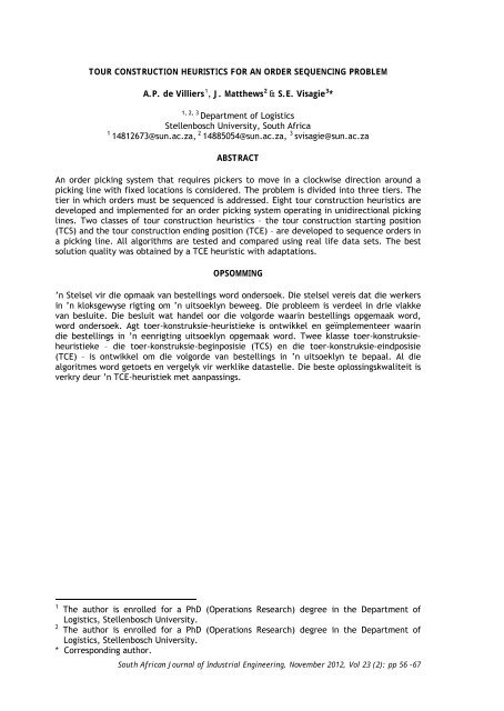
TOUR CONSTRUCTION HEURISTICS FOR AN ORDER SEQUENCING PROBLEM
A.P. de Villiers 1 , J. Matthews 2 & S.E. Visagie 3 *
1, 2, 3
Department of Logistics
Stellenbosch University, South Africa
1
14812673@sun.ac.za, 2 14885054@sun.ac.za, 3 svisagie@sun.ac.za
ABSTRACT
An order picking system that requires pickers to move in a clockwise direction around a
picking line with fixed locations is considered. The problem is divided into three tiers. The
tier in which orders must be sequenced is addressed. Eight tour construction heuristics are
developed and implemented for an order picking system operating in unidirectional picking
lines. Two classes of tour construction heuristics – the tour construction starting position
(TCS) and the tour construction ending position (TCE) – are developed to sequence orders in
a picking line. All algorithms are tested and compared using real life data sets. The best
solution quality was obtained by a TCE heuristic with adaptations.
OPSOMMING
’n Stelsel vir die opmaak van bestellings word ondersoek. Die stelsel vereis dat die werkers
in ’n kloksgewyse rigting om ’n uitsoeklyn beweeg. Die probleem is verdeel in drie vlakke
van besluite. Die besluit wat handel oor die volgorde waarin bestellings opgemaak word,
word ondersoek. Agt toer-konstruksie-heuristieke is ontwikkel en geïmplementeer waarin
die bestellings in ’n eenrigting uitsoeklyn opgemaak word. Twee klasse toer-konstruksieheuristieke
– die toer-konstruksie-beginposisie (TCS) en die toer-konstruksie-eindposisie
(TCE) – is ontwikkel om die volgorde van bestellings in ’n uitsoeklyn te bepaal. Al die
algoritmes word getoets en vergelyk vir werklike datastelle. Die beste oplossingskwaliteit is
verkry deur ’n TCE-heuristiek met aanpassings.
A
A
A
A
A
A
A
A
A
A
A
A
A
A
A
A
A
A
A
a
1 The author is enrolled for a PhD (Operations Research) degree in the Department of
Logistics, Stellenbosch University.
2 The author is enrolled for a PhD (Operations Research) degree in the Department of
Logistics, Stellenbosch University.
* Corresponding author.
South African Journal of Industrial Engineering, November 2012, Vol 23 (2): pp 56 -67

1. BACKGROUND AND INTRODUCTION
Order picking is known to be the most important activity in distribution centres (DCs) [19].
It involves the process of retrieving products from storage (or buffer areas) in response to a
specific customer request [3]. Usually, more than one order picking system is used in a DC.
These order picking systems may be fully automated or operated by humans, but most
systems employ humans as order pickers. In a typical DC, about 65% of operating expenses
are consumed by order picking [15]. The organisation of order picking operations impacts
on the DC’s performance, and therefore also on that of the supply chain [3]. DC design,
storage assignment, and picker route planning may be used to enhance operating efficiency
and space utilisation to reduce order picking costs [9].
The order picking system in a DC owned by Pep Stores Ltd (‘Pep’), located in South Africa,
is considered in this paper. Pep is a chain store operating more than 1,500 branches. Pep
specialises in clothing but also sells other products, including home accessories and cellular
phones. Orders processed by the DC are requests for specific branches. An order for a retail
outlet is a set of products, together with the quantity of each product required by that
retail outlet. The size of the products has a direct impact on the picking system used by
Pep.
The DC uses an order picking system that is based on the concept of a wave. A wave may be
described as the set of stock keeping units (SKUs) in conjunction with the set of branches
requiring at least one of the SKUs. All the orders for that wave are picked as a single
operation. All the SKUs in a wave are therefore completely picked for all branches during
that wave.
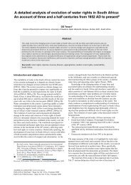
To pick each wave, the DC uses a picking line. Figure 1 is a schematic representation of a
typical picking line used in the DC. An SKU is stored in a single location, and only SKUs
within the same wave may be stored on the same picking line. Pickers move in a clockwise
direction around the conveyor belt, picking the required SKUs for each order.
Figure 1: A schematic representation of the physical layout of a picking line containing
m locations
A voice-automated software system is used to communicate instructions to the pickers. This
system directs each picker to the required locations for a single order. Once a picker has
picked all the SKUs in an order, the voice-automated software system will direct the picker
to the closest required SKU for a new order. The system ensures that a picker will complete
all the picks for a single order before starting a new order. This system ensures that pickers
pick orders sequentially.
Each day picking lines are identified that will become available for waves during that
specific day. SKUs are then identified and grouped in the waves scheduled for the available
57

picking lines. A first-in-first-out (FIFO) policy is used to determine the SKUs that have to be
scheduled. The set of SKUs in a wave are then assigned to the available picking lines. Once
all the SKUs to be placed in a picking line are known, they are assigned specific locations
based on in-house guidelines. When the picking line becomes available, each SKU is
retrieved from storage and placed in its designated location. Once all the SKUs have been
placed, order picking may begin.
The planning of picking lines may be divided into three tiers of decisions. The first tier
determines which SKUs should be allocated to which picking line. The problem of assigning
scheduled SKUs to available picking lines is referred to as the ‘SKU to Picking Line
Assignment Problem’ (SPLAP). The second tier, known as the ‘SKU to Location Problem’
(SLP), considers the positioning of the various SKUs in a picking line. The final tier considers
the sequencing of the orders for pickers within a picking line, and is referred to as the
‘Order Sequencing Problem’ (OSP). All of these subproblems aim to achieve the objective of
picking all the orders in the shortest possible time.
The decisions associated with each tier are made sequentially during the planning of a
picking line. First it has to be decided which SKUs are assigned to which picking lines; then
each SKU has to be assigned to a specific location in the picking line; and finally the
sequence in which the orders should be picked must be determined.
Each subproblem therefore relies on the information generated by its predecessor. Thus, to
solve a subproblem the solution to the successive subproblem must be known. For example,
to evaluate a candidate solution for an instance of the SLP, the optimum sequencing of
orders generated by the OSP is required. Due to this exchange of information between
subproblems, the first subproblem which needs to be solved is the OSP. Any alteration in
the SLP or the SPLAP will influence the OSP. Since the OSP must be tested repetitively for
various alterations to the SLP or SPLAP, the OSP has to be solved quickly to avoid incurring
significantly high overall computational times.
2. THE OSP
The OSP may be described as the sequencing of all the orders, for each picker, given a
wave of SKUs assigned to distinct locations in a picking line, such that the total picking time
is minimised.
Each order requires a number of distinct SKUs in various amounts. A picker must visit each
location containing the SKUs required by that order and collect for each SKU the requested
number of units of that SKU. A picker may only start a new order once all the SKUs have
been collected from the current order. Pickers are required to move in a clockwise
direction when collecting SKUs.
The following assumptions are derived from consultation with Pep’s DC management and
from the assumptions of Matthews & Visagie [11].
1. A picker must complete an entire order before starting another. The next order
may not start at the same location where the previous order ended.
2. The time taken physically to pick an SKU is constant with regard to all the orders.
3. A picker walks at a more-or-less constant speed.
4. An order may start at any location, and will finish at the last location where an
SKU is picked for that order.
5. The time required to switch to the next order is negligible.
Given these assumptions, the OSP may be viewed as an equality-generalised travelling
salesman problem (E-GTSP). The E-GTSP partitions nodes into clusters, and the problem
calls for a minimum cost cycle visiting exactly one node in each cluster [5]. The E-GTSP is
an NP-hard problem [8].
58

If a cluster is defined as all possible starting positions associated with an order, each order
(cluster) must be followed by another order (cluster). Additionally only a single starting
location (node) in each order (cluster) must be selected.
Let the duple (i, l) represent order l starting at location i. Let N be a set of all duples (i, l)
and I 1 I 2 , … , I m a proper partition of the set N, where I l = {(1, l), (2, l), … , (m, l)}, if m
locations are present on a single picking line. The set N may be interpreted as the vertices
on a digraph, with edges representing the distance in number of locations between orders.
The time needed to pick a product from a location is considered to be constant. The time
needed to travel between orders and locations is considered to be variable. Thus the
objective is to sequence a set of orders in such a way as to minimise the total distance
travelled, and therefore the total travel time, to complete all the orders.
Following the formulation by De Villiers & Visagie [4], let
and
p k
f(x) = 1, if order k starting at location i is followed by order l
0, otherwise
be the position of order k within the order sequence.
The following parameters are set in the model. Let
n
be the total number of order,
m
be the total number of locations,
d ik
be the number of locations which must be passed to complete
order k starting at location i and
e ijk =
1, if orderk starting at location i is completed at location j
0, otherwise
The objective is then to
subject to
m
m
minimise d ik x ikl
m
n
n
i=1 k=1 l=1
m
n
x ikl = 1
i=1 l=1
m n
x ikl = 1
i=1 k=1
m
n
x i1l = 0
i=2
x ikl − x pqk e pqi ≤ 0
l=1
p=1 q=1
(1)
l = 1, … , n, (2)
k = 1, … , n, (3)
l = 1, … , n, (4)
i = 1, … , m,
k = 1, … , n,
p 1 = 1, (6)
m
p k − p l + n x ikl ≤ n − 1
k = 1, … , n,
l = 2, … , n,
(7)
i=1
(5)
x ikl ∈ {0,1}
i = 1, … , m,
k = 1, … , n,
(8)
l = 1, … , n,
p k ≥ 0 k = 1, … , n, (9)
59

The objective function (1) minimises the total distance travelled by a picker. Constraint
sets (2) and (3) ensure that each order is completed only once. Constraint sets (4) and (6)
ensure that the first order (which is a dummy order) is completed first and that it starts at
location 1. Constraint set (5) ensures that if order k starts at location i then the order that
precedes order k will end at location i. For example, if order k (starting at location i)
follows order q (starting at location p), then order q should end at location i. Therefore if
x ikl equals 1 then both e pqi and x pqk should also equal 1. Constraint set (7) follows from the
standard MTZ constraints [14]. It ensures that no subtours are generated. Subtours will
occur if at least two subsets of orders form their own closed pick sequences. One closed
pick sequence containing all the orders must be determined. The size of this formulation is
n 2 m + n variables (of which n 2 m are binary) and n 2 + 2n + nm constraints. For a typical
real life instance n ≈ 1 200 and m ≈ 56, yielding a number of variables in excess of 8 × 10 7
and a number of constraints in excess of 1,5 × 10 6 , which renders an exact approach
impossible.
Matthews & Visagie [11] suggested a maximal cut approach to solve this problem. This
approach always leads to a solution within one picking cycle of a lower bound to the
problem. However, the computational times for a typical real life instance of the model are
more than five minutes if solved on an Intel® Core TM 2 Duo 3GHz with 3.7 GB RAM running
Windows XP [18] using Lingo 11 [12]. The computational time for this approach is too long
for use in solving the SLP where many different SKU locations must be tested. Faster
approaches are therefore required to solve the OSP in less computational time. In the next
section, a short section on heuristic approaches in general is presented. However, this
paper focuses on tour construction heuristics to solve the OSP in much shorter times, while
maintaining reasonable solution quality.
3. HEURTISTICS FOR TSPs
TSP heuristics are typically classified into three types: tour construction heuristics, tour
improvement heuristics, and randomised improvement heuristics. Combinations of these
approaches are also found in the literature [6]. Typical tour construction heuristics include
the nearest neighbour heuristic, the family of insertion heuristic, Clark and Wright savings
heuristic, the minimal spanning tree heuristic, and Christofides’ heuristic [6,7]. Tour
improvement heuristics take a feasible solution to the TSP and improve on that solution by
locally changing the sequence in which nodes are visited. A well-known tour improvement
heuristic is the k-opt method, which replaces k arcs in the solution by another set of k arcs
that will result in a better solution [1]. Most randomised tour improvement heuristics arise
from the subject of metaheuristics, which includes algorithms like tabu search, simulated
annealing, genetic algorithms, and ant colony optimisation to solve TSPs [2].
The OSP presented here is not well suited to tour improvement or randomised improvement
heuristics, nor even to a combination of these methods. Both of these approaches start with
a current tour and attempt to improve on it by performing local changes to it. The
structure of the OSP limits the use of tour improvement heuristics, as a change in the
ending position of an order may effect all starting and ending positions (and thus pick
distances) of subsequent orders in the sequence. Therefore, by changing the sequence in
which a subset of orders is picked, the quality of the sequence of orders that follows this
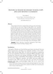
changed subset also changes. This characteristic is illustrated by an example picking line
with ten locations and four orders. Figure 2 (a) illustrates the order sequence (A, B, C, D, E)
with a total pick length of 32 locations. The individual pick lengths of each order are also
given. If the sequence is changed by moving order D to the start of the sequence, as shown
in Figure 2 (b), both orders A and D will have shorter pick lengths, implying a local
improvement on orders A and D. The end location of order A is changed, however, and the
pick lengths for orders C and D have now increased, resulting in a longer total pick
distance. Although only one order was moved in the sequence (it is a local change) the pick
lengths for all the following orders changed. Therefore only tour construction heuristics
that add on orders at the end of the sequence are suitable for this variant of the TSP.
60

Experiments with real life data confirm that the problem shown in the example above holds
in general. Tour improvement heuristics and randomised improvement heuristics yield
substantially inferior results to tour construction heuristics, and are thus not considered
further in this paper.
Figure 2: An example of a picking line with ten locations and four orders. A letter in a
location indicates that a specific order require SKUs from that location.
4. TOUR CONSTRUCTION APPROACHES
The general framework of tour construction heuristics has been adapted to take the
structure of the problem into account. To explain the approaches presented here, a number
of definitions are required [11].
Let a span of an order be the smallest set of locations passed to pick the entire order, given
a starting location. A span for an order k starting at location i may be represented by
S k i = 〈i, e k i 〉, where i is the starting location and e k
i
the closest ending location of order k.
Any starting location for an order has a unique span associated with it, since an order must
be completed once it is started.
Let the size of a span be the number of locations traversed to complete the order picked on
that span. Each order may be assigned a starting point from all the possible locations within
i
a picking line. The size of a span S k for an order k may be represented by:
S i k = 〈i, e i k
〉 = e k i i
− i if i < e k
m + e i i
k − i if i ≥ e k
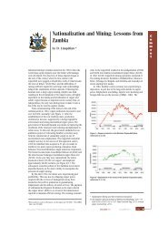
where m is the total number of locations. Consider the example in Figure 3, where order k
requires SKUs from locations 9, 12 and 16. If a picker who is currently at location 6 is
assigned order k he will traverse a distance of S 6 k = |〈6,16〉| = 10 locations and end at
location 16. The locations traversed by the picker are indicated by the thick dashed line in
Figure 3. Furthermore, let P k be the number of different SKUs that are required by order k.
For the example in Figure 3, three SKUs are picked in order k, resulting in P k = 3.
Let the minimum span S k
min
of an order be a span of smallest size for an order. From the
example in Figure 3, S k min = |〈9,16〉| = 7.
The tour construction heuristics presented here attempt to assign a desirable order to a
picker when he/she finishes his/her current order. The influence of this assignment on the
sequence of future orders is not considered.
61

Figure 3: A schematic representation of the layout of a picking line containing 20
locations. The squares indicates the SKUs that are requested by an order k.
4.1 Tour construction starting heuristic
The tour construction starting heuristic (TCS) considers the starting location of preferable
orders. If any orders require an SKU from the current location of the picker, only these
orders are considered. The order with the shortest span is then selected for picking. When
the picker has completed the order, the current location of the picker is updated
accordingly.
If, however, no orders require an SKU at the current location, the current location is
incremented by one until an order is found that does require an SKU from the current
location. This process is repeated iteratively until all orders are picked. The general
framework of the TCS is given in Algorithm 1.
Algorithm 1: Tour construction starting heuristic (TCS)
The TCS therefore determines the next order, k, to be picked from location i as
k = arg min
k∈R i
S k i , (10)
where R i is the set of orders, not yet completed, that have to be picked from location i. If
R i = ∅, the current location i is increased by one. The nearest order may be interpreted as
the order that may be completed within the smallest number of locations from the current
location.
4.2 Tour construction ending heuristic
The tour construction ending heuristic (TCE) considers the end location of pending orders if
started at the current location of picker i. The spans of all pending orders starting at
location i are used as a measure, and the order with the shortest span is selected. The
general framework of the TCE is given in Algorithm 2.
62

Algorithm 2: Tour construction ending heuristic (TCE)
The next order in the TCE is determined as
k = arg min
k∈U S k i , (11)
where U is the set of uncompleted orders. The TCE heuristic essentially considers all
uncompleted orders, whereas the TCS considers only a subset of these for selection.
4.3 Results of the tour construction heuristic approaches
To evaluate the proposed tour construction heuristics, 22 real-life data sets were received
from Pep. The heuristics were compared with a lower bound obtained by the maximal cut
approach described by Matthews & Visagie [11]. All the algorithms were tested using an
Intel® Core TM 2Duo 3 GHz with 3.7 GB RAM running Linux Ubuntu 9.10 [17] using Java [16].
The average time for solving an instance by means of the maximal cut approach is about
five minutes. Both the heuristics were tested, and all computation times were significantly
less than one second, which is significantly lower than the maximal cut approach.
The data sets were divided into three groups: large, medium, and small. Large data sets
have more than 1,000 orders, medium data sets contain between 200 and 1,000 orders, and
small data sets less than 200 orders. Table 1 displays the results for the various heuristics,
as well as the lower bound.
The TCS outperformed the TCE for the large data sets. The TCE, however, outperforms the
TCS for the medium and small data sets.
Table 1: Results obtained from the TCS and TCE used to solve several OSP instances.
The solutions are displayed as the number of cycles traversed to pick all the orders. The best
performing heuristic for each data set is indicated in boldface. The size – that is, number of orders
(O) and locations (L) – is displayed for each data set.
63

5. TOUR CONSTRUCTION HEURISTIC ADAPTATIONS
Focusing solely on spans as a way to distinguish between desirable orders may be
inadequate. This is illustrated by an example, shown in Figure 4, with a picking line
containing two orders: order k (indicated by squares) and order l (indicated by triangles).
Figure 4: A schematic representation of the layout of a picking line containing 20
locations.
The squares indicate the SKUs that are requested by an order k, where triangles indicate the SKUs
that are required by an order l.
Consider a picker currently positioned at location 4. Either order k or order l may be
picked. There is no preference between the two orders as S 4 k = S 4 l = |〈4,16〉| = 12. The
minimum span of order k, however, is S 4 k . In this situation it may be more desirable to pick
order k, as the picker is able to pick it on its minimum span, leaving order l for a later
opportunity when the picker might pick order l on a shorter span too. In the next section,
adaptations of the TCS and TCE are introduced to address this situation.
5.1 Minimum span adaptations
In an effort to assign preference to picking orders on their minimum spans, the length of a
proposed span of an order is compared with the length of its minimum span. Both the TCS
and the TCE were adapted with this variation (TCS 1 and TCE 1 ). Let the TCS 1 determine the
next order k to be picked, given a current location $i$, to be sequenced as
S i k
k = arg min
k∈R i S min k .
If S i k S min k the pick-length of order k is at a minimum. Similarly, the next order k
sequenced in the TCE 1 given a current location i is determined as
k = arg min
k∈U
S i k
S min k .
5.2 Pick density adaptations
A situation may arise where multiple orders have identical spans given a starting location,
but the number of picks may differ. This variation uses a similar approach to TCS 1 and
TCE 1 , but considers the number of picks in an order instead of the minimum span. Let the
TCS 2 heuristic determine the next order k to be picked to be
S i k
k = arg min ,
k∈R i P k
where i is the current location and P k is the number of picks in order k. If S i k ⁄ P k the picklength
of order k is at a minimum and there is a pick at each location on the minimum
span. The next order in the TCE 2 heuristic is determined as
S i k
k = arg min .
k∈U P k
64

5.3 Combined relative measures
A final approach is considered where the combined influences of the relative measures are
used. This variation combines the relative measures of considering the minimum span of an
order, as well as the number of picks in an order. Let the TCS 3 heuristic determine the next
order k to be picked as
S i k
k = arg min
k∈R i S min .
k ∙ P k
The next order in the TCE 3 heuristic is determined as
S i k
k = arg min
k∈U S min .
k ∙ P k
This variation considers both the minimum span and the number of possible starting
locations for each order. An adaptation, where the denominator in TCS 3 and TCE 3 may be
altered to the additive form, was also tested. This approach delivers similar results to the
multiplicative case.
5.4 Results of the adapted tour construction heuristic approaches
Table 2 displays the results obtained for all the variations of the TCS and TCE heuristics
used to solve the OSP. The TCE heuristic and its variations outperform the TCS heuristic and
its variations. This may be attributed to the fact that the TCE heuristics consider a wider
range of possible orders to be picked when selecting a following order.
Table 2: Results obtained from all the variations of the TCS and TCE heuristics used to
solve the OSP.
A total of 22 real-life data sets are considered where the number of orders (O) and locations (L)
are displayed for each data set. The solutions displayed in bold type indicate the best-performing
heuristic for each data set.
Table 3 displays the computational times for all the tour construction heuristics considered
in this paper. The computational times are given in milliseconds.
In an effort to compare algorithms over multiple data sets, the results of each algorithm
were normalised relative to the lower bound. The data were normalised by dividing the
number of cycles traversed by the lower bound. This normalisation establishes a relative
measure by which algorithms may be compared. The normalised results for each size of
data were then grouped as one sample of elements, and the testing was done to determine
whether there were significant differences in the mean between the different algorithms.
65

An overall level of significance in the form of a Bonferroni t-test was performed for the 22
instances considered, to determine if the mean solution of one instance differs significantly
between all possible pairs of instances. In the case where x instances are considered
x = x(x − 1) ⁄ 2 two sample t-tests may be performed to test for significant difference
2
between all possible pairs of instances.
Table 3: Computational times in milliseconds for all the variations of the TCS and TCE
heuristics used to solve the OSP.
A total of 22 real life data sets are considered where number of orders (O) and locations (L) are
displayed for each data set.
The Bonferroni method may overcome the problem of assigning an overall level of
significance when considering a large number of t-tests. The confidence level is modified
from α to 2α⁄ x(x − 1) for each of the t-tests. The confidence level then pertains to each of
the x(x − 1) ⁄ 2 confidence intervals covering their respective differences of population
means [10]. The confidence level helps to determine if statistically significant differences
are large enough to be of practical importance.
Table 4 shows the results obtained when a Bonferroni t-test was conducted on the
performance of the average of the solution quality of each heuristic divided by the lower
bound for each data set [10]. The different classes indicate that the means of various
heuristics considered were significantly different for a Bonferroni multiple comparison test
with p < 0.05.
On average, the TCE 3 heuristic performs best for small data sets, while TCE 2 performs best
for medium and large data sets. The TCS heuristics and its variations are comprehensively
outperformed by the solutions of the TCE heuristic and its variations.
6. CONCLUSION
An order picking operation found in a DC owned by Pep Stores was investigated. Three tiers
of problems were identified: the SPLAP, SLP, and OSP. Quick tour construction heuristics
are required to solve the OSP, since the SLP and SPLAP can only be solved by repeatedly
solving the OSP. Initially two classes of tour construction heuristics were introduced,
followed by extensions of these heuristics. Computational results are presented that
illustrate the improved performance when extending the original heuristics. The bestperforming
heuristic is the TCE with relative measures. In particular, the TCE 2 achieved the
best overall performance of the instances considered.
66

Table 4: Results obtained from the Bonferroni t-test for small, medium and large data sets.
The mean represents the average of the results obtained by the respective heuristics divided by
the lower bound. The value of N indicates the number of observations considered for each class.
REFERENCES
[1] Barun, C., Karloff, H. & Tovey, C. 1999. New results on the old k-opt algorithm for the traveling
salesman problem, Operations Research, 28(6), pp. 1998-2029.
[2] Cheng, C.B. & Mao, C.P. 2007. A modified ant colony system for solving the travelling salesman
problem with time windows, Mathematical and Computer Modelling, 46(9-10), pp. 1225-1235.
[3] De Koster, R., Le-Duc, T. & Roodbergen, K.J. 2007. Design and control of warehouse order
picking: A literature review, European Journal of Operational Research, 182(2), pp. 481-501.
[4] De Villiers, A.P. & Visagie, S.E. 2011. Toewysingsheuristieke om die volgorde van bestellings vir
’n uitsoeklyn te bepaal, Litnet Akademies, 9(1) pp. 1-22.
[5] Fischetti, M., González, J.J.S. & Toth P. 1997. A branch-and-cut algorithm for the symmetric
generalized traveling salesman problem, Operations Research, 45(3), pp. 378-394.
[6] Gendreau, M., Hertz, A. & Laporte, G. 1992. New insertion and postoptimisation procedures for
the traveling salesman problem, SIAM Journal on Computing, 40(6), pp. 1086-1094.
[7] Johnson, D.S. & McGeoch, L.A. 2007. Experimental analysis of heuristics for the STSP, in Gutin,
G. & Punnen, A.P. (eds), The traveling salesman problem and its variations, Springer, New York,
pp. 369-443.
[8] Gutin, G. & Yeo, A. 2003. Assignment problem based algorithms are impractical for the
generalized TSP, Australasian Journal of Combinatorics, 27, pp. 149-153.
[9] Hsieh, L. & Tsai, L. 2006. The optimum design of a warehouse system on order picking
efficiency, The International Journal of Advanced Manufacturing Technology, 28(5-6), pp. 626-
637.
[10] Johnson, R.A. 2005. Miller & Freund’s probability and statistics for engineers, 7 th ed., Pearson
Prentice Hall.
[11] Matthews, J. & Visagie, S.E. 2011. Order sequencing on a unidirectional cyclical picking line,
[Submitted].
[12] Lindo Systems. 2011. Lingo 11. Retrieved March 2011 from www.lindo.com.
[13] Litvak, N. & Vlasiou, M. 2009. A survey on performance analysis of warehouse carousel systems,
(Unpublished) Technical Report, Department of Applied Mathematics, University of Twente,
Twente.
[14] Punnen, A.P. 2007. The traveling salesman problem: Applications, formulations and variations,
in Gutin, G. & Punnen, A.P. (eds), The traveling salesman problem and its variations, Springer,
New York, pp. 1-28.
[15] Ruben, R.A. & Jacobs, F.R. 1999. Batch construction heuristics and storage assignment
strategies for walk/ride and pick systems, Management Science, 45(4), pp. 575-596.
[16] Sun Microsystems. 2011. Java. Retrieved June 2011 from http://java.sun.com.
[17] Ubuntu. 2011. Retrieved March 2011 from www.ubuntu.com.
[18] Microsoft. 2011. Windows XP. Retrieved March 2011 from www.microsoft.com.
[19] Yu, M. & de Koster, R.B.M. 2009. The impact of order batching and picking area zoning on order
picking system performance, European Journal of Operational Research, 198(2), pp. 480-490.
67