Numerical Differentiation First Derivative Second Derivative Error ...

More documents

Recommendations

Info

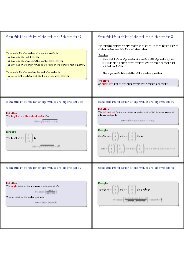
Richardson Extrapolation III Summary It is an estimate for f ′ (x) whose truncation error is O(h 4 ), and so is an improvement over D 0 used alone. This technique of using calculations with different h values to get a better estimate is known as Richardson Extrapolation. Richardson’s Extrapolation. Suppose that we have the two approximations D 0 (h) and D 0 (2h) for f ′ (x), then an improved approximation has the form: f ′ (x) = 4D 0(h) − D 0 (2h) + O(h 4 ) 3 Approximation for numerical differentiation: Approximation for f ′ (x) Error Forward/backward difference D + , D − O(h) Central difference D 0 O(h 2 ) Richardson Extrapolation O(h 4 ) Considering the total error (approximation error + calculation error): |R| ≤ f ′′′ ∣ (ξ) ∣∣∣ ∣ h 2 + ∣ ǫ ∣ 6 h remember that h should not be chosen too small. Solving Differential Equations Numerically Working Example Definition. The Initial value Problem deals with finding the solution y(x) of y ′ = f(x, y) with the initial condition y(x 0 ) = y 0 It is a 1st order differential equations (D.E.s). 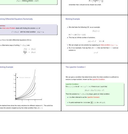Alternative ways of writing y ′ = f(x, y) are: y ′ (x) = f(x, y) dy(x) dx = f(x, y) We shall take the following D.E. as an example: f(x, y) = y or y ′ = y (or y ′ (x) = y(x)). This has an infinite number of solutions: y(x) = C · e x ∀C ∈ R We can single out one solution by supplying an initial condition y(x 0 ) = y 0 . So, in our example, if we say that y(0) = 1, then we find that C = 1 and out solution is y = e x Working Example The Lipschitz Condition I y 30 - Initial Condition 25 20 15 10 5 x 1 0 1 2 3 The dashed lines show the many solutions for different values of C. The solid line shows the solution singled out by the initial condition that y(0) = 1. We can give a condition that determines when the initial condition is sufficient to ensure a unique solution, known as the Lipschitz Condition. Lipschitz Condition: For a ≤ x ≤ b, for all −∞ < y, y ∗ < ∞, if there is an L such that |f(x, y) − f(x, y ∗ )| ≤ L |y − y ∗ | Then the solution to y ′ = f(x, y) is unique, given an initial condition. L is often referred to as the Lipschitz Constant. A useful estimate for L is to take ∣ ∂f ∂y∣ ≤ L, for x in (a, b).
The Lipschitz Condition II Numerically solving y ′ = f(x, y) Example. given our example of y ′ = y = f(x, y), then we can see do we get a suitable L. So we shall try L = 1 ∂f ∂y = ∂(y) ∂(y) = 1 |f(x, y) − f(x, y ∗ )| = |y − y ∗ | ≤ 1 · |y − y ∗ | So we see that we satisfy the Lipschitz Condition with a Constant L = 1. We assume we are trying to find values of y for x ranging over the interval [a, b]. We start with the one point where we have the exact answer, namely the initial condition y 0 = y(x 0 ). We generate a series of x-points from a = x 0 to b, separated by a small step-interval h: x 0 = a x i = a + i · h ∣ h = b−a N x N = b we want to compute {y i }, the approximations to {y(x i )}, the true values. Euler’s Method Euler’s Method The technique works by using applying f at the current point (x n , y n ) to get an estimate of y ′ at that point. Euler’s Method. This is then used to compute y n+1 as follows: y n+1 = y n + h · f(x n , y n ) This technique for solving D.E.’s is known as Euler’s Method. Example. In our example, we have y ′ = y f(x, y) = y y n+1 = y n + h · y n At each point after x 0 , we accumulate an error, because we are using the slope at x n to estimate y n+1 , which assumes that the slope doesn’t change over interval [x n , x n+1 ]. It is simple, slow and inaccurate, with experimentation showing that the error is O(h). Truncation Errors I Definitions. The error introduced at each step is called the Local Truncation Error. The error introduced at any given point, as a result of accumulating all the local truncation errors up to that point, is called the Global Truncation Error. y(x ) n+1 y n y n+1 Truncation Errors II We can estimate the local truncation error y(x n+1 ) − y n+1 , by assuming the value y n for x n is exact as follows: as follows: Using Taylor Expansion about x = x n y(x n+1 ) = y(x n + h) y(x n+1 ) = y(x n ) + hy ′ (x n ) + h2 2 y′′ (ξ) Assuming y n is exact (y n = y(x n )), so y ′ (x n ) = f(x n , y n ) y(x n+1 ) = y n + hf(x n , y n ) + h2 2 y′′ (ξ) Now looking at y n+1 by definition of the Euler method: x n x n+1 In the diagram above, the local truncation error is y(x n+1 ) − y n+1 . We subtract the two results: y n+1 = y n + hf(x n , y n ) y(x n+1 ) − y n+1 = − h2 2 y′′ (ξ)
Page 1 and 2: Numerical Differentiation First Der
Page 3: Rounding Error in Difference Equati
Page 7: Runge-Kutta Techniques II Runge-Kut

Numerical Differentiation First Derivative Second Derivative Error ...

You also want an ePaper? Increase the reach of your titles

Delete template?

Save as template?