Numerical Differentiation First Derivative Second Derivative Error ...
Numerical Differentiation First Derivative Second Derivative Error ...
Numerical Differentiation First Derivative Second Derivative Error ...

You also want an ePaper? Increase the reach of your titles
YUMPU automatically turns print PDFs into web optimized ePapers that Google loves.
<strong>Numerical</strong> <strong>Differentiation</strong><br />
<strong>First</strong> <strong>Derivative</strong><br />
We assume that we can compute a function f , but that we have no information about<br />
how to compute f ′ . We want ways of estimating f ′ (x), given what we know about f .<br />
Reminder: definition of differentiation:<br />
df<br />
dx = lim f(x + ∆x) − f(x)<br />
∆x→0 ∆x<br />
For second derivatives, we have the definition:<br />
d 2 f<br />
dx 2 = lim f ′ (x + ∆x) − f ′ (x)<br />
∆x→0 ∆x<br />
We can use this formula, by taking ∆x equal to some small value h, to get the following<br />
approximation,<br />
known as the Forward Difference (D + (h)):<br />
f ′ (x) ≈ D + (h) =<br />
f(x + h) − f(x)<br />
h<br />
Alternatively we could use the interval on the other side of x, to get the Backward<br />
Difference (D − (h)) :<br />
f ′ f(x) − f(x − h)<br />
(x) ≈ D − (h) =<br />
h<br />
A more symmetric form, the Central Difference (D 0 (h)), uses intervals on either<br />
side of x:<br />
f ′ f(x + h) − f(x − h)<br />
(x) ≈ D 0 (h) =<br />
2h<br />
All of these give (different) approximations to f ′ (x).<br />
<strong>Second</strong> <strong>Derivative</strong><br />
<strong>Error</strong> Estimation in <strong>Differentiation</strong> I<br />
We shall see that the error involved in using these differences is a form of truncation<br />
error (R T ):<br />
= D + (h) − f ′ (x)<br />
R T<br />
= 1 h (f(x + h) − f(x)) − f ′ (x)<br />
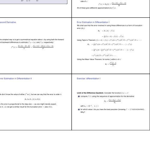
The simplest way is to get a symmetrical equation about x by using both the forward<br />
and backward differences to estimate f ′ (x + ∆x) and f ′ (x) respectively:<br />
f ′′ (x) ≈ D +(h) − D − (h)<br />
h<br />
=<br />
f(x + h) − 2f(x) + f(x − h)<br />
h 2<br />
Using Taylor’s Theorem: f(x + h) = f(x) + f ′ (x)h + f ′′ (x)h 2 /2! + f (3) (x)h 3 /3! + · · · :<br />
R T = 1 h (f ′ (x)h + f ′′ (x)h 2 /2! + f ′′′ (x)h 3 /3! + · · · ) − f ′ (x)<br />
= 1 h f ′ (x)h + h 1(f ′′ (x)h 2 /2! + f ′′′ (x)h 3 /3! + · · · )) − f ′ (x)<br />
= f ′′ (x)h/2! + f ′′′ (x)h 2 /3! + · · ·<br />
Using the Mean Value Theorem, for some ξ within h of x:<br />
R T = f ′′ (ξ) · h<br />
2<br />
<strong>Error</strong> Estimation in <strong>Differentiation</strong> II<br />
Exercise: differentiation I<br />
We don’t know the value of either f ′′ or ξ, but we can say that the error is order h:<br />
R T for D + (h) is O(h)<br />
so the error is proportional to the step size — as one might naively expect.<br />
For D − (h) we get a similar result for the truncation error — also O(h).<br />
Limit of the Difference Quotient. Consider the function f(x) = e x .<br />
1 compute f ′ (1) using the sequence of approximation for the derivative:<br />
with h k = 10 −k , k ≥ 1<br />
D k = f(x + h k) − f(x)<br />
h k<br />
2 for which value k do you have the best precision (knowing e 1 = 2.71828182845905).<br />
Why?
Exercise: differentiation II<br />
Central Difference<br />
1 xls/Lect13.xls<br />
2 Best precision at k = 8. When h k is too small, f(1) and f(1 + h k ) are very close<br />
together. The difference f(1 + h k ) − f(1) can exhibit the problem of loss of<br />
significance due to the substraction of quantities that are nearly equal.<br />
we have looked at approximating f ′ (x) with the backward D − (h) and forward<br />
difference D + (h).<br />
Now we just check out the approximation with the central difference:<br />
f ′ (x) ≃ D 0 (h) =<br />
f(x + h) − f(x − h)<br />
2h<br />
Richardson extrapolation<br />
<strong>Error</strong> analysis of Central Difference I<br />
<strong>Error</strong> analysis of Central Difference II<br />
We consider the error in the Central Difference estimate (D 0 (h)) of f ′ (x):<br />
We apply Taylor’s Theorem,<br />
D 0 (h) =<br />
f(x + h) = f(x) + f ′ (x)h + f ′′ (x)h 2<br />
2!<br />
f(x − h) = f(x) − f ′ (x)h + f ′′ (x)h 2<br />
f(x + h) − f(x − h)<br />
2h<br />
2!<br />
+ f ′′′ (x)h 3<br />
3!<br />
− f ′′′ (x)h 3<br />
3!<br />
(A) − (B) = 2f ′ (x)h + 2 f ′′′ (x)h 3<br />
3!<br />
(A) − (B)<br />
= f ′ (x) + f ′′′ (x)h 2<br />
2h<br />
3!<br />
+ f (4) (x)h 4<br />
4!<br />
+ f (4) (x)h 4<br />
4!<br />
+ 2 f (5) (x)h 5<br />
5!<br />
+ f (5) (x)h 4<br />
5!<br />
+ · · · (A)<br />
+ · · · (B)<br />
+ · · ·<br />
+ · · ·<br />
We see that the difference can be written as<br />
or alternatively, as<br />
D 0 (h) = f ′ (x) + f ′′ (x)<br />
6<br />
where be know how to compute b 1 , b 2 , etc.<br />
h 2 + f (4) (x)<br />
+ · · ·<br />
24<br />
D 0 (h) = f ′ (x) + b 1 h 2 + b 2 h 4 + · · ·<br />
We see that the error R T = D 0 (h) − f ′ (x) is O(h 2 ).<br />
Remark. Remember: for D − and D + , the error is O(h).<br />
<strong>Error</strong> analysis of Central Difference III<br />
Rounding <strong>Error</strong> in Difference Equations I<br />
Example.<br />
Let try again the example:<br />
f(x) = e x<br />
We evaluate f ′ (1) = e 1 ≈ 2.71828... with<br />
for h = 10 −k , k ≥ 1.<br />
D 0 (h) =<br />
<strong>Numerical</strong> values: xls/Lect13.xls<br />
f ′ (x) = e x<br />
f(1 + h) − f(1 − h)<br />
2h<br />
When presenting the iterative techniques for root-finding, we ignored rounding<br />
errors, and paid no attention to the potential error problems with performing<br />
subtraction. This did not matter for such techniques because:<br />
1 the techniques are self-correcting, and tend to cancel out the accumulation of rounding<br />
errors<br />
2 the iterative equation x n+1 = x n − c n where c n is some form of correction factor has a<br />
subtraction which is safe because we are subtracting a small quantity (c n) from a large<br />
one (e.g. for Newton-Raphson, c n = f(x)<br />
f ′ (x) ).
Rounding <strong>Error</strong> in Difference Equations II<br />
Rounding <strong>Error</strong> in Difference Equations III<br />
However, when using a difference equation like<br />
D 0 (h) =<br />
f(x + h) − f(x − h)<br />
2h<br />
we seek a situation where h is small compared to everything else, in order to get a<br />
good approximation to the derivative. This means that x + h and x − h are very<br />
similar in magnitude, and this means that for most f (well-behaved) that f(x + h)<br />
will be very close to f(x − h). So we have the worst possible case for subtraction:<br />
the difference between two large quantities whose values are very similar.<br />
We cannot re-arrange the equation to get rid of the subtraction, as this difference<br />
is inherent in what it means to compute an approximation to a derivative<br />
(differentiation uses the concept of difference in a deeply intrinsic way).<br />
We see now that the total error in using D 0 (h) to estimate f ′ (x) has two<br />
components<br />
1 the truncation error R T which we have already calculated,<br />
2 and a function calculation error R XF which we now examine.<br />
When calculating D 0 (h), we are not using totally accurate computations of f , but<br />
instead we actually compute an approximation ¯f , to get<br />
¯D 0 (h) = ¯f(x + h) − ¯f(x − h)<br />
2h<br />
We shall assume that the error in computing f near to x is bounded in magnitude<br />
by ǫ:<br />
|¯f(x) − f(x)| ≤ ǫ<br />
Rounding <strong>Error</strong> in Difference Equations IV<br />
The calculation error is then given as<br />
R XF = ¯D 0 (h) − D 0 (h)<br />
= ¯f(x + h) − ¯f(x − h) f(x + h) − f(x − h)<br />
−<br />
2h<br />
2h<br />
= ¯f(x + h) − ¯f(x − h) − (f(x + h) − f(x − h))<br />
2h<br />
= ¯f(x + h) − f(x + h) − (¯f(x − h) − f(x − h))<br />
2h<br />
|R XF| ≤ |¯f(x + h) − f(x + h)| + |¯f(x − h) − f(x − h)|<br />
2h<br />
≤<br />
ǫ + ǫ<br />
2h<br />
≤<br />
ǫ h<br />
So we see that R XF is proportional to 1/h, so as h shrinks, this error grows, unlike<br />
R T which shrinks quadratically as h does.<br />
Rounding <strong>Error</strong> in Difference Equations V<br />
We see that the total error R is bounded by |R T| + |R XF|, which expands out to<br />
|R| ≤<br />
f ′′′ ∣<br />
(ξ) ∣∣∣ ∣ h 2 + ∣ ǫ ∣<br />
6 h<br />
So we see that to minimise the overall error we need to find the value of h = h opt which<br />
minimises the following expression:<br />
Unfortunately, we do not know f ′′′ or ξ !<br />
f ′′′ (ξ)<br />
h 2 + ǫ 6 h<br />
Many techniques exist to get a good estimate of h opt , most of which estimate f ′′′<br />
numerically somehow. These are complex and not discussed here.<br />
Richardson Extrapolation I<br />
Richardson Extrapolation II<br />
The trick is to compute D 0 (h) for 2 different values of h, and combine the results in<br />
some appropriate manner, as guided by our knowledge of the error behaviour.<br />
In this case we have already established that<br />
D 0 (h) =<br />
f(x + h) − f(x − h)<br />
2h<br />
We now consider using twice the value of h:<br />
D 0 (2h) =<br />
We can subtract these to get:<br />
f(x + 2h) − f(x − 2h)<br />
4h<br />
= f ′ (x) + b 1 h 2 + O(h 4 )<br />
= f ′ (x) + b 1 4h 2 + O(h 4 )<br />
D 0 (2h) − D 0 (h) = 3b 1 h 2 + O(h 4 )<br />
The righthand side of this equation is simply D 0 (h) − f ′ (x), so we can substitute to get<br />
D 0 (2h) − D 0 (h)<br />
3<br />
This re-arranges (carefully) to obtain<br />
f ′ (x)<br />
= D 0 (h) − f ′ (x) + O(h 4 )<br />
= D 0 (h) + D0(h)−D0(2h)<br />
3 + O(h 4 )<br />
= 4D0(h)−D0(2h)<br />
3 + O(h 4 )<br />
We divide across by 3 to get:<br />
D 0 (2h) − D 0 (h)<br />
3<br />
= b 1 h 2 + O(h 4 )
Richardson Extrapolation III<br />
Summary<br />
It is an estimate for f ′ (x) whose truncation error is O(h 4 ), and so is an<br />
improvement over D 0 used alone.<br />
This technique of using calculations with different h values to get a better estimate<br />
is known as Richardson Extrapolation.<br />
Richardson’s Extrapolation.<br />
Suppose that we have the two approximations D 0 (h) and D 0 (2h) for f ′ (x), then an<br />
improved approximation has the form:<br />
f ′ (x) = 4D 0(h) − D 0 (2h)<br />
+ O(h 4 )<br />
3<br />
Approximation for numerical differentiation:<br />
Approximation for f ′ (x)<br />
<strong>Error</strong><br />
Forward/backward difference D + , D − O(h)<br />
Central difference D 0 O(h 2 )<br />
Richardson Extrapolation O(h 4 )<br />
Considering the total error (approximation error + calculation error):<br />
|R| ≤<br />
f ′′′ ∣<br />
(ξ) ∣∣∣ ∣ h 2 + ∣ ǫ ∣<br />
6 h<br />
remember that h should not be chosen too small.<br />
Solving Differential Equations <strong>Numerical</strong>ly<br />
Working Example<br />
Definition.<br />
The Initial value Problem deals with finding the solution y(x) of<br />
y ′ = f(x, y) with the initial condition y(x 0 ) = y 0<br />
It is a 1st order differential equations (D.E.s).<br />
Alternative ways of writing y ′ = f(x, y) are:<br />
y ′ (x) = f(x, y)<br />
dy(x)<br />
dx<br />
= f(x, y)<br />
We shall take the following D.E. as an example:<br />
f(x, y) = y<br />
or y ′ = y (or y ′ (x) = y(x)).<br />
This has an infinite number of solutions:<br />
y(x) = C · e x ∀C ∈ R<br />
We can single out one solution by supplying an initial condition y(x 0 ) = y 0 .<br />
So, in our example, if we say that y(0) = 1, then we find that C = 1 and out<br />
solution is<br />
y = e x<br />
Working Example<br />
The Lipschitz Condition I<br />
y<br />
30<br />
- Initial Condition<br />
25<br />
20<br />
15<br />
10<br />
5<br />
x<br />
1<br />
0<br />
1 2 3<br />
The dashed lines show the many solutions for different values of C. The solid line<br />
shows the solution singled out by the initial condition that y(0) = 1.<br />
We can give a condition that determines when the initial condition is sufficient to<br />
ensure a unique solution, known as the Lipschitz Condition.<br />
Lipschitz Condition:<br />
For a ≤ x ≤ b, for all −∞ < y, y ∗ < ∞, if there is an L such that<br />
|f(x, y) − f(x, y ∗ )| ≤ L |y − y ∗ |<br />
Then the solution to y ′ = f(x, y) is unique, given an initial condition.<br />
L is often referred to as the Lipschitz Constant.<br />
A useful estimate for L is to take ∣ ∂f<br />
∂y∣ ≤ L, for x in (a, b).
The Lipschitz Condition II<br />
<strong>Numerical</strong>ly solving y ′ = f(x, y)<br />
Example.<br />
given our example of y ′ = y = f(x, y), then we can see do we get a suitable L.<br />
So we shall try L = 1<br />
∂f<br />
∂y<br />
= ∂(y)<br />
∂(y)<br />
= 1<br />
|f(x, y) − f(x, y ∗ )| = |y − y ∗ |<br />
≤ 1 · |y − y ∗ |<br />
So we see that we satisfy the Lipschitz Condition with a Constant L = 1.<br />
We assume we are trying to find values of y for x ranging over the interval [a, b].<br />
We start with the one point where we have the exact answer, namely the initial<br />
condition y 0 = y(x 0 ).<br />
We generate a series of x-points from a = x 0 to b, separated by a small<br />
step-interval h:<br />
x 0 = a<br />
x i = a + i · h<br />
∣ h = b−a<br />
N<br />
x N = b<br />
we want to compute {y i }, the approximations to {y(x i )}, the true values.<br />
Euler’s Method<br />
Euler’s Method<br />
The technique works by using applying f at the current point (x n , y n ) to get an<br />
estimate of y ′ at that point.<br />
Euler’s Method.<br />
This is then used to compute y n+1 as follows:<br />
y n+1 = y n + h · f(x n , y n )<br />
This technique for solving D.E.’s is known as Euler’s Method.<br />
Example.<br />
In our example, we have<br />
y ′ = y f(x, y) = y y n+1 = y n + h · y n<br />
At each point after x 0 , we accumulate an error, because we are using the slope at x n to<br />
estimate y n+1 , which assumes that the slope doesn’t change over interval [x n , x n+1 ].<br />
It is simple, slow and inaccurate, with experimentation showing that the error is<br />
O(h).<br />
Truncation <strong>Error</strong>s I<br />
Definitions.<br />
The error introduced at each step is called the Local Truncation <strong>Error</strong>.<br />
The error introduced at any given point, as a result of accumulating all the local<br />
truncation errors up to that point, is called the Global Truncation <strong>Error</strong>.<br />
y(x ) n+1<br />
y n<br />
y n+1<br />
Truncation <strong>Error</strong>s II<br />
We can estimate the local truncation error y(x n+1 ) − y n+1 , by assuming the value y n for<br />
x n is exact as follows: as follows:<br />
Using Taylor Expansion about x = x n<br />
y(x n+1 ) = y(x n + h)<br />
y(x n+1 ) = y(x n ) + hy ′ (x n ) + h2<br />
2 y′′ (ξ)<br />
Assuming y n is exact (y n = y(x n )), so y ′ (x n ) = f(x n , y n )<br />
y(x n+1 ) = y n + hf(x n , y n ) + h2<br />
2 y′′ (ξ)<br />
Now looking at y n+1 by definition of the Euler method:<br />
x n<br />
x n+1<br />
In the diagram above, the local truncation error is y(x n+1 ) − y n+1 .<br />
We subtract the two results:<br />
y n+1 = y n + hf(x n , y n )<br />
y(x n+1 ) − y n+1 = − h2<br />
2 y′′ (ξ)
Truncation <strong>Error</strong>s III<br />
Introduction<br />
So<br />
y(x n+1 ) − y n+1 ∝ O(h 2 )<br />
We saw that the local truncation error for Euler’s Method is O(h 2 ).<br />
By integration (accumulation of error when starting from x 0 ), we see that global<br />
error is O(h).<br />
As a general principle, we find that if the Local Truncation <strong>Error</strong> is O(h p+1 ), then the<br />
Global Truncation <strong>Error</strong> is O(h p ).<br />
Considering the problem of solving differential equations with one initial condition, we<br />
learnt about:<br />
Lipschitz Condition (unicity of the solution)<br />
finding numerically the solution : Euler method<br />
Today is about how to improve the Euler’s algorithm:<br />
Heun’s method<br />
and more generally Runge-Kutta’s techniques.<br />
Improved <strong>Differentiation</strong> Techniques I<br />
Improved <strong>Differentiation</strong> Techniques II<br />
We can improve on Euler’s technique to get better estimates for y n+1 . The idea is to<br />
use the equation y ′ = f(x, y) to estimate the slope at x n+1 as well, and then average<br />
these two slopes to get a better result.<br />
k1<br />
(e)<br />
y n<br />
y n+1<br />
0.5(k1+k2)<br />
x n<br />
y n+1<br />
x n+1<br />
k2<br />
Using the slope y ′ (x n , y n ) = f(x n , y n ) at x n , the Euler approximation is:<br />
(A)<br />
y n+1 − y n<br />
h<br />
≃ f(x n , y n )<br />
Considering the slope y ′ (x n+1 , y n+1 ) = f(x n+1 , y n+1 ) at x n+1 , we can propose this<br />
new approximation:<br />
(B)<br />
y n+1 − y n<br />
h<br />
≃ f(x n+1 , y n+1 )<br />
The trouble is: we dont know y n+1 in f (because this is what we are looking for!).<br />
So instead we use y (e)<br />
n+1 the Euler’s approximation of y n+1:<br />
(B)<br />
y n+1 − y n<br />
h<br />
≃ f(x n+1 , y (e)<br />
n+1 )<br />
Improved <strong>Differentiation</strong> Techniques III<br />
Runge-Kutta Techniques I<br />
So considering the two approximations of yn+1−yn<br />
h with expressions (A) and (B), we get<br />
a better approximation by averaging (ie. by computing A+B/2):<br />
Heun’s Method.<br />
The approximation:<br />
y n+1 − y n<br />
h<br />
y n+1 = y n + h 2 ·<br />
is known as Heun’s Method.<br />
≃ 1 (<br />
2 · f(x n , y n ) + f(x n+1 , y (e) )<br />
n+1<br />
(<br />
f(x n , y n ) + f(x n+1 , y (e) )<br />
n+1<br />
= y n + h 2 · (f(x n, y n ) + f(x n+1 , y n + h · f(x n , y n ))<br />
It can be shown to have a global truncation error that is O(h 2 ). The cost of this<br />
improvement in error behaviour is that we evaluate f twice on each h-step.<br />
We can repeat the Heun’s approach by considering the approximations of slopes<br />
in the interval [x n ; x n+1 ].<br />
This leads to a large class of improved differentiation techniques which evaluate f<br />
many times at each h-step, in order to get better error performance.<br />
This class of techniques is referred to collectively as Runge-Kutta techniques, of<br />
which Heun’s Method is the simplest example.<br />
The classical Runge-Kutta technique evaluates f four times to get a method with<br />
global truncation error of O(h 4 ).
Runge-Kutta Techniques II<br />
Runge-Kutta’s technique using 4 approximations.<br />
It is computed using approximations of the slope at x n , x n+1 and also two<br />
approximations at mid interval x n + h 2 :<br />
with<br />
y n+1 − y n<br />
h<br />
= 1 6 (f 1 + 2 · f 2 + 2 · f 3 + f 4 )<br />
f 1 = f (x n , y n)<br />
(<br />
)<br />
f 2 = f x n + h 2 , y n + h 2 f 1<br />
(<br />
)<br />
f 3 = f x n + h 2 , y n + h 2 f 2<br />
f 4 = f (x n+1 , y n + h · f 3 )<br />
It can be shown that the global truncation error is O(h 4 ).