Testcase 3.7 DNS and LES of transitional flow around a high lift ...
Testcase 3.7 DNS and LES of transitional flow around a high lift ...
Testcase 3.7 DNS and LES of transitional flow around a high lift ...

You also want an ePaper? Increase the reach of your titles
YUMPU automatically turns print PDFs into web optimized ePapers that Google loves.
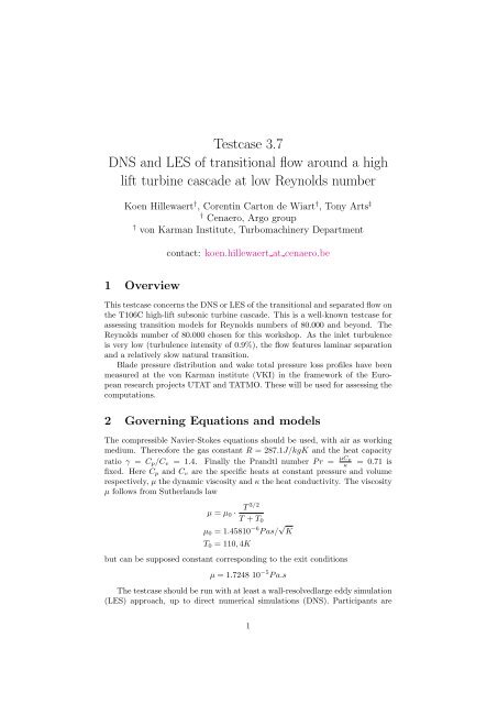
<strong>Testcase</strong> <strong>3.7</strong><br />
<strong>DNS</strong> <strong>and</strong> <strong>LES</strong> <strong>of</strong> <strong>transitional</strong> <strong>flow</strong> <strong>around</strong> a <strong>high</strong><br />
<strong>lift</strong> turbine cascade at low Reynolds number<br />
Koen Hillewaert † , Corentin Carton de Wiart † , Tony Arts ‡<br />
† Cenaero, Argo group<br />
† von Karman Institute, Turbomachinery Department<br />
contact: koen.hillewaert at cenaero.be<br />
1 Overview<br />
This testcase concerns the <strong>DNS</strong> or <strong>LES</strong> <strong>of</strong> the <strong>transitional</strong> <strong>and</strong> separated <strong>flow</strong> on<br />
the T106C <strong>high</strong>-<strong>lift</strong> subsonic turbine cascade. This is a well-known testcase for<br />
assessing transition models for Reynolds numbers <strong>of</strong> 80.000 <strong>and</strong> beyond. The<br />
Reynolds number <strong>of</strong> 80.000 chosen for this workshop. As the inlet turbulence<br />
is very low (turbulence intensity <strong>of</strong> 0.9%), the <strong>flow</strong> features laminar separation<br />
<strong>and</strong> a relatively slow natural transition.<br />
Blade pressure distribution <strong>and</strong> wake total pressure loss pr<strong>of</strong>iles have been<br />
measured at the von Karman institute (VKI) in the framework <strong>of</strong> the European<br />
research projects UTAT <strong>and</strong> TATMO. These will be used for assessing the<br />
computations.<br />
2 Governing Equations <strong>and</strong> models<br />
The compressible Navier-Stokes equations should be used, with air as working<br />
medium. There<strong>of</strong>ore the gas constant R = 287.1J/kgK <strong>and</strong> the heat capacity<br />
ratio γ = C p /C v = 1.4. Finally the Pr<strong>and</strong>tl number P r = µCp<br />
κ<br />
= 0.71 is<br />
fixed. Here C p <strong>and</strong> C v are the specific heats at constant pressure <strong>and</strong> volume<br />
respectively, µ the dynamic viscosity <strong>and</strong> κ the heat conductivity. The viscosity<br />
µ follows from Sutherl<strong>and</strong>s law<br />
T 3/2<br />
µ = µ 0 ·<br />
T + T 0<br />
µ 0 = 1.45810 −6 P as/ √ K<br />
T 0 = 110, 4K<br />
but can be supposed constant corresponding to the exit conditions<br />
µ = 1.7248 10 −5 P a.s<br />
The testcase should be run with at least a wall-resolvedlarge eddy simulation<br />
(<strong>LES</strong>) approach, up to direct numerical simulations (<strong>DNS</strong>). Participants are<br />
1
obviously free concerning the choice <strong>of</strong> models, but are expected to provide<br />
details on the model itself as well as the specificities <strong>of</strong> the implementation in<br />
relation to the discretisation method. Participants are allowed to complete the<br />
results with wall-modeled <strong>LES</strong> (WM<strong>LES</strong>) or other hybrids <strong>of</strong> <strong>LES</strong>.<br />
3 Flow Conditions<br />
The low Reynolds number is obtained during the measurements by lowering the<br />
pressure in the closed loop tunnel [1]. The conditions are derived in A, <strong>and</strong> are<br />
summarized as:<br />
• inlet total pressure p t = 7198.5P a;<br />
• inlet total temperature T t = 298.15K;<br />
• pitchwise inlet <strong>flow</strong> angle 32.7 ◦ from the axial direction;<br />
• the exit static pressure p 2 = 5419.3P a<br />
4 Geometry <strong>and</strong> grids<br />
The geometry <strong>of</strong> the T106C blade is shown in figure 1 <strong>and</strong> available as a set<br />
<strong>of</strong> ordered points running <strong>around</strong> the blade; their location is shown in figure<br />
2. Furthermore a basic Gmsh geometry <strong>and</strong> meshing description is available<br />
which constructs an extruded mesh over a spanwise extent <strong>of</strong> S = 0.2C. Also<br />
IGS/STEP/PARASOLID <strong>of</strong> the 2D <strong>and</strong> 3D geometry can be obtained.<br />
5 M<strong>and</strong>atory results<br />
The following results will be used for quantitative assessment<br />
• the time- <strong>and</strong> spanwise averaged static pressure distribution on the blade<br />
as function <strong>of</strong> the axial distance with respect to the axial chord. This<br />
distance is measured between the vertical tangents at the front <strong>and</strong> aft <strong>of</strong><br />
the blade;<br />
• the total pressure distribution in the wake, measured at an axial distance<br />
<strong>of</strong> 0.465C ax downstream <strong>of</strong> the vertical tangent <strong>of</strong> the aft <strong>of</strong> the blade;<br />
• the mean exit <strong>flow</strong> angle measured at the same position.<br />
The following results are requested for further qualitative discussion<br />
• the rms <strong>and</strong> correlations <strong>of</strong> the velocity fluctuations on the spanwise periodic<br />
plane;<br />
• the rms <strong>of</strong> the pressure fluctuations on the surface;<br />
• the time-averaged skin-friction on the blade;<br />
• the time-averaged vorticity on the spanwise periodic plane;<br />
• the time-averaged total pressure on the spanwise periodic plane;<br />
2
Figure 1: Geometrical description <strong>of</strong> the blade section (Courtesy VKI)<br />
3
Figure 2: Point distribution<br />
• a snapshot <strong>of</strong> the vorticity ω x , ω y <strong>and</strong> ω z components on the spanwise<br />
periodic plane;<br />
• a snapshot <strong>of</strong> the skin friction on the blade at the same time.<br />
6 Reference data<br />
The reference data include static pressure distributions on the blade surface, as<br />
well as total pressure distribution in the wake, <strong>and</strong> have been measured at the<br />
von Karman Institute. The results have been partially published in [1].<br />
4
Isentropic Mach number distribution along the blade for several Reynolds numbers at M 2,is = 0.65<br />
1<br />
0.9<br />
0.8<br />
M is<br />
0.7<br />
0.6<br />
0.5<br />
0.4<br />
250000<br />
0.3<br />
TRAF<br />
0.2<br />
0.1<br />
0<br />
0.0 0.1 0.2 0.3 0.4 0.5 0.6 0.7 0.8 0.9 1.0<br />
X / C ax<br />
80000<br />
100000<br />
120000<br />
140000<br />
160000<br />
185000<br />
210000<br />
0.10<br />
0.09<br />
0.08<br />
0.07<br />
0.06<br />
0.05<br />
0.04<br />
83500<br />
101000<br />
119000<br />
141000<br />
160000<br />
185500<br />
210000<br />
250000<br />
0.03<br />
0.02<br />
0.01<br />
0.00<br />
0.0 0.1 0.2 0.3 0.4 0.5 0.6 0.7 0.8 0.9 1.0<br />
5
References<br />
[1] Jan Michálek, Michelangelo Monaldi,Tony Arts, Aerodynamic Performance<br />
<strong>of</strong> a Very High Lift Low Pressure Turbine Airfoil (T106C) at Low Reynolds<br />
<strong>and</strong> High Mach Number With Effect <strong>of</strong> Free Stream Turbulence Intensity,<br />
ASME Journal <strong>of</strong> Turbomachinery, volume 134, november 2012<br />
A<br />
Derivation <strong>of</strong> the physical conditions<br />
The working gas is air, hence R = 287.1 J/kgK <strong>and</strong> γ = 1.4. The total<br />
inlet temperature is fixed at T t = 298.15K, whilst the the isentropic exit Mach<br />
number is fixed as M 2s = 0.65. Consequently, we find<br />
• exit static temperature<br />
T 2s =<br />
T t<br />
1 + γ−1<br />
2 M = 274.92K<br />
2s<br />
2<br />
• exit dynamic viscosity as given by Sutherl<strong>and</strong>s law<br />
µ 2s = 1.458 × 10 −6 T 3/2<br />
2s<br />
T 2s + 110.4 = 1.7248 × 10⁻⁵ P a.s<br />
• exit velocity v 2s = M 2s<br />
√ γRT2s = 216.07 m/s<br />
• outlet isentropic density from the Reynolds number Re 2s = 80.000 <strong>and</strong><br />
the chord C = 0.09301<br />
ρ 2s = Re 2sµ 2s<br />
v 2s C<br />
= 0.0687 kg/m3<br />
• inlet total pressure follows from the outlet pressure p 2s <strong>and</strong> the exit Mach<br />
number M 2s<br />
p 2s = ρ 2s RT 2s = 5419.3P a<br />
(<br />
p t = p 2s · 1 + γ − 1 ) γ<br />
M2s<br />
2 γ−1<br />
= 7198.5P a<br />
2<br />
6